The Slope-Deflection Method: A Two-Span Steel Beam Solved by Hand
The slope-deflection method makes the joint rotations the unknowns, writes every member end moment as a function of them, and solves an indeterminate structure the way your software does internally. We solve a two-span continuous steel beam end to end by hand, every number confirmed on a real FEM engine, with a free live calculator.
Key takeaways
- The slope-deflection method is a displacement method: it makes the joint rotations the unknowns, writes each member end moment as (2EI/L)(2θn + θf − 3ψ) + FEM, imposes equilibrium at every joint, and solves. It is the hand ancestor of the stiffness matrix your software runs.
- The applied load enters only through fixed-end moments: wL²/12 for a uniform load, PL/8 for a central point load, both signed clockwise-positive. The rest of the method corrects those clamped-joint moments for the rotation the joints actually undergo.
- For our two-span beam, three joint rotations collapse to a single unknown, EIθB = −36 kN·m², giving a hogging 72 kN·m over the interior support and reactions of 48, 120 and 12 kN that sum to the 180 kN total load.
- In a prismatic continuous beam EI cancels: the moments are purely geometric, set by span lengths and loads. EI only matters for unequal member stiffness, for the actual deflections, or when a support settles.
- The −3ψ chord-rotation term absorbs support settlement and frame sway directly, the feature that makes slope-deflection worth learning: it is what a finite element solver does when it forms and solves Ku = F, which reproduced every hand number here to three decimals.
Solve an indeterminate beam by hand, the way your software does it inside
Somewhere in the second half of a structural analysis course, Estruturas I or Análise Estrutural or whatever your curriculum calls it, the subject stops being about drawing free bodies and starts being about a harder question: how do you find the forces in a beam that statics alone cannot solve? The first complete answer most students meet is the slope-deflection method, and it earns every hour you spend on it, because it is the exact idea your analysis software runs millions of times a second without ever telling you.
The method has one governing idea. Instead of chasing forces, you make the displacements the unknowns: the rotations of the joints. You write each member's end moments as a function of those rotations, you impose equilibrium at every joint, and you solve a small set of linear equations for the rotations. Back-substitute, and every end moment falls out. That is the whole method, and it is the hand ancestor of the stiffness matrix.
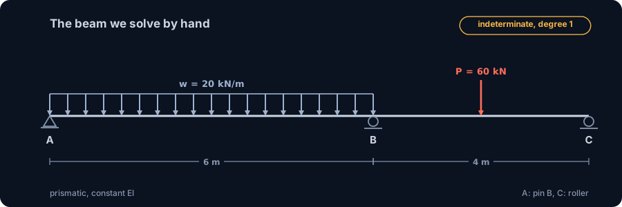
This guide solves one problem completely: a two-span continuous steel beam, unequal spans, a distributed load on one and a point load on the other. We set it up, count its indeterminacy, write the slope-deflection equations, solve the joint rotations, and read off the moments. Then we hand the identical beam to the finite element engine that ships inside CalcSteel and watch it reproduce every number to three decimals. There is a live calculator on the page so you can drive it yourself.
We wrote it for three readers. If you are a student, this is the worked example that finally makes the method click. If you are a practising or self-employed calculista, it is the sanity check behind the black box, the thing that lets you trust, or catch, what the software returns. And if you have only ever pressed Analyze, this is what the software is actually doing.
What the slope-deflection method actually is
The slope-deflection method is a displacement method: it treats the unknown joint rotations, and when a frame can sway the joint translations too, as the primary unknowns, and expresses every member end moment as a linear function of them. This is the opposite of the force methods, virtual work or the flexibility method, which take redundant forces as the unknowns. Choosing displacements is what makes it scale, and what makes it the direct ancestor of matrix and finite element analysis.
Three quantities appear in every slope-deflection calculation, and getting them straight is most of the method:
- Joint rotations θ. Each rigid joint rotates by some angle under load. These are the unknowns you solve for. A continuous beam on simple supports has one rotation unknown at each interior support, and one at each simple end until you simplify them away.
- Fixed-end moments (FEM). The moments a span would develop at its ends if both ends were perfectly clamped, computed from the load alone. They are the starting point: the applied load enters the method only through the FEMs.
- Member stiffness 2EI/L. How hard a member resists having its ends rotated. Stiffer or shorter members attract more moment, which is why an indeterminate structure shares load by relative stiffness.
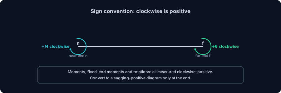
The sign convention is not optional and not negotiable. Clockwise member-end moments are positive. Every end moment, every fixed-end moment, every rotation is measured with the same clockwise-positive rule, and the single most common way to wreck a slope-deflection solution is to let a sagging-positive bending convention leak into it halfway through. Keep the two apart: solve in clockwise-positive member moments, then convert to a sagging-positive bending moment diagram only at the very end.
Where the method came from, and where it went
The slope-deflection method is not a modern trick. It is a specific historical bridge between hand statics and the computer, and knowing the lineage tells you why it looks the way it does.
- 1880, Heinrich Manderla writes member end moments in terms of end rotations to compute secondary stresses in truss joints, the first appearance of the core idea.
- 1892, Otto Mohr and Emil Winkler develop it further, still in the setting of secondary stresses in framed structures.
- 1914, Axel Bendixen applies the displacement idea systematically to rigid frames and gives the method its name: the slope-deflection method.
- 1915, George A. Maney presents it in the form still taught today for rigid-jointed structures, and it becomes a standard method of analysis in the United States.
- 1930, Hardy Cross publishes moment distribution, an iterative way to solve the very same joint-equilibrium equations without inverting a matrix by hand, and it dominates design offices for a generation.
- 1950s to 60s, matrix structural analysis and the finite element method generalise the slope-deflection equations into the stiffness matrix. Every rotation unknown becomes a degree of freedom, every 2EI/L becomes an entry in K, and the joint-equilibrium equations become Ku = F.
This is the punchline to carry through the rest of the article: when a finite element solver assembles its stiffness matrix and solves for nodal rotations, it is doing exactly what you are about to do by hand, only with more degrees of freedom and no arithmetic slips. The slope-deflection method is the readable source code of the black box.
The slope-deflection equation, term by term
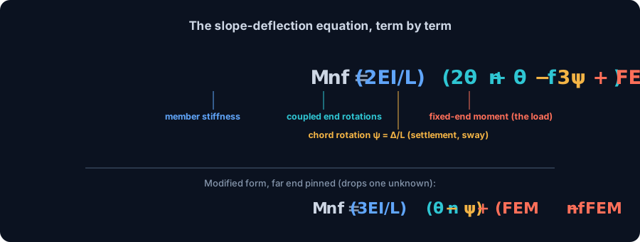
Everything reduces to one equation, written once for each end of each member. For a member spanning from a near end n to a far end f, the moment at the near end is:
Mnf = (2EI / L)(2θn + θf − 3ψ) + FEMnf
Read it term by term, because each term is a physical effect:
- (2EI / L) is the member's rotational stiffness. Long soft members contribute little, short stiff ones dominate.
- 2θn + θf couples the two ends. Rotating the near end raises its own moment twice as much as rotating the far end does, the 2-to-1 carry-over that also shows up in moment distribution as a carry-over factor of one half.
- − 3ψ is the chord rotation term, where ψ = Δ / L is the rigid-body rotation of the member axis caused by one end settling, or the frame swaying, by Δ. On a beam with no support movement, ψ = 0 and the term vanishes. It is the term that lets slope-deflection handle settlement and sway directly, which the pure force methods cannot do as cleanly.
- FEMnf is the fixed-end moment at that end, the only place the applied load enters.
There is one simplification worth its weight in gold. When the far end of a member is a simple support, a pin or roller with a known zero moment, you can eliminate its rotation in advance and use the modified slope-deflection equation:
Mnf = (3EI / L)(θn − ψ) + (FEMnf − FEMfn / 2)
This drops one unknown per pinned end, and it is why a continuous beam with simple ends collapses to just the interior-support rotations. We use both forms below so you can watch them agree.
Fixed-end moments: how the load gets in
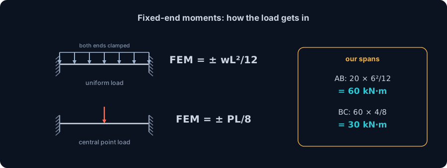
The load never touches a rotation directly. It enters only through the fixed-end moments, the moments each span would develop at its ends if both ends were fully clamped against rotation. You look them up, and for the two loads in our problem they are the two most common cases in every table:
- Uniform load w over a span L: FEM = ± wL² / 12, counterclockwise (negative) at the left end and clockwise (positive) at the right end.
- Central point load P on a span L: FEM = ± PL / 8, with the same sign pattern.
For our beam that gives, before any rotation is known:
- Span AB, w = 20 kN/m, L = 6 m: FEMAB = − 20 × 6² / 12 = − 60 kN·m, FEMBA = + 60 kN·m.
- Span BC, P = 60 kN, L = 4 m: FEMBC = − 60 × 4 / 8 = − 30 kN·m, FEMCB = + 30 kN·m.
Notice what the fixed-end moments are: the moments in a world where the joints cannot rotate. The real structure is not that world, so its joints do rotate, and the slope-deflection equations are the bookkeeping that corrects the fixed-end moments for the rotation the joints actually undergo. That is the entire logic in one sentence.
Worked example: the two-span beam, solved end to end
Now the whole method on one structure. Continuous beam A-B-C: pin at A, roller at B, roller at C, prismatic with constant EI. Span AB = 6 m carries a uniform w = 20 kN/m, span BC = 4 m carries a central P = 60 kN.
Step 1, count the unknowns
Three supports on a continuous beam with simple ends: the count gives a degree of static indeterminacy of one, one redundant, which you can take as the moment over the interior support. In displacement terms the free rotations are θA, θB, θC. We solve the full set of three, then show the one-unknown shortcut gives the same answer.
Step 2, write the four member end moments
Using Mnf = (2EI / L)(2θn + θf) + FEM with ψ = 0 (no support movement), and writing a = EIθA, b = EIθB, c = EIθC to keep the algebra clean:
- MAB = (2EI/6)(2θA + θB) − 60 = (2a + b)/3 − 60
- MBA = (2EI/6)(2θB + θA) + 60 = (2b + a)/3 + 60
- MBC = (2EI/4)(2θB + θC) − 30 = (2b + c)/2 − 30
- MCB = (2EI/4)(2θC + θB) + 30 = (2c + b)/2 + 30
Step 3, impose joint equilibrium
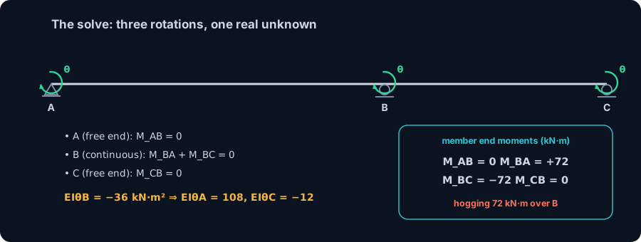
At each support the member end moments must balance the applied joint moment, which is zero here. A and C are simple ends carrying a single member, so their end moment is zero. B is continuous, so the two member moments there must sum to zero:
- Joint A: MAB = 0 ⇒ 2a + b = 180
- Joint C: MCB = 0 ⇒ 2c + b = − 60
- Joint B: MBA + MBC = 0 ⇒ 2a + 10b + 3c = − 180
Step 4, solve the rotations
From the A and C equations, a = 90 − b/2 and c = − 30 − b/2. Substitute both into the B equation and everything collapses to one unknown: 270 + 7.5b = 0, so EIθB = b = − 36 kN·m². Back out the others: EIθA = 108 and EIθC = − 12 kN·m². The rotations depend on EI, but the moments will not, because EI cancels in a prismatic beam.
Step 5, back-substitute for the moments
Put the rotations back into the four equations:
- MAB = (2×10⁸ − 36)/3 − 60 = 180/3 − 60 = 0 (as it must be, A is a free end)
- MBA = (2×(−36) + 108)/3 + 60 = 36/3 + 60 = + 72 kN·m
- MBC = (2×(−36) − 12)/2 − 30 = −84/2 − 30 = − 72 kN·m
- MCB = (2×(−12) − 36)/2 + 30 = −60/2 + 30 = 0 (C is a free end)
Joint B checks: +72 and −72 sum to zero. The interior support carries a hogging moment of 72 kN·m, and that single number is the redundant the count told us to expect. The one-unknown shortcut, using the modified 3EI/L equation on both pinned-ended spans, gives the identical EIθB = −36 and the identical 72 kN·m, which is the fastest way to check your algebra.
Try it: watch the interior support attract the moment
The fastest way to feel the method is to build the beam yourself and watch the redistribution happen. The calculator below is the real CalcSteel beam tool, live on this page. Start with a single simply supported span and read the tidy parabolic moment. Then add an interior support to make the beam continuous, and watch a hogging moment appear over that support while the span moments drop: that hogging value is exactly the redundant the slope-deflection method solves for.
Change the span lengths so they are unequal, like our 6 and 4, and the symmetry breaks the way it does in the worked example: the shorter, stiffer span pulls more moment toward the joint. Every number the tool shows comes from the same stiffness equations you just solved by hand, only assembled into a matrix instead of written out.
It is the real thing, free, with no login for the math. If it opens in its own tab, here is the direct link to the free beam calculator, and its companion the shear and moment diagram calculator draws the full diagrams for any span and load.
Max moment
45 kN·m
Max shear
30 kN
Max deflection
10.55 mm
= L/569
Bending stress σ
84.4 MPa
σ = M/Sx
Utilization
44.0%
NBR 8800 · δ ≤ L/250
Geometry & supports
Section
Ix 7999 cm⁴ · Sx 533 cm³ · 42.2 kg/m
Point loads (↓ positive)
None — add as many as you need.
Distributed loads (uniform or trapezoidal)
Model sketch
Diagrams — free PNG / SVG / CSV export, no watermark
Step-by-step — the calculation memory of YOUR beam
IPE 300 · L = 6 m · fy = 250 MPa
1. Reactions (equilibrium of the solved FEM model)
ΣFy = 0 · ΣM = 0
R_A = 30 kN · R_B = 30 kN
2. Peak shear (read from the SFD)
Vmax = |V(x)|max
Vmax = -30 kN @ x = 6 m
3. Peak moment (read from the BMD)
Mmax = |M(x)|max
Mmax = 45 kN·m @ x = 3 m
4. Peak deflection
EI = 15998 kN·m² (E = 200 GPa)
δmax = 10.55 mm @ x = 3 m = L/569
5. Elastic bending stress
σ = Mmax / Sx = 45.00 × 10³ / 533.3
σ = 84.4 MPa
6. Bending check — both codes, side by side
NBR 8800: σ ≤ fy/1.10 = 227.3 MPa · AISC 360: σ ≤ 0.90·fy = 225 MPa
NBR 37.1% PASS · AISC 37.5% PASS
7. Deflection check (serviceability — code-independent)
δ ≤ L/250 = 24 mm
10.55 mm / 24 mm = 44.0% PASS
Recomputed live from the current inputs by the direct-stiffness FEM engine — change any load and every step updates. Reproduce it by hand with the formulas in the sections below.
Lightest catalog profiles that pass (974 flexural candidates · NBR 8800)
| Profile | Std | Weight | Total steel | σ util | δ util | |
|---|---|---|---|---|---|---|
| W310x21 | AISC | 21 kg/m | 126 kg | 83% | 98% | |
| VS 300x23 | BR | 22.6 kg/m | 136 kg | 71% | 84% | |
| U 300x90x6.3 | BR | 23.1 kg/m | 139 kg | 82% | 98% | |
| U 300x100x6.3 | BR | 24.1 kg/m | 145 kg | 77% | 91% | |
| VS 250x25 | BR | 24.6 kg/m | 148 kg | 70% | 100% |
Elastic bending (σ = M/Sx vs fy/γa1, γa1 = 1.10 — NBR 8800) + deflection screening of the full flexural catalog. Lateral-torsional buckling, shear and local buckling are NOT checked here — run the full NBR 8800 / AISC 360 verification in the 3D editor.
From end moments to reactions and the diagram
The end moments are the hard part. Everything after them is statics. With the interior support moment known, cut the beam at B into two simply supported spans, each carrying the 72 kN·m hogging moment at its B end, and take moments.
Reactions
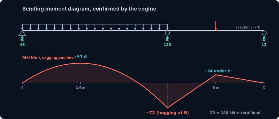
For span AB the uniform load alone splits 60 kN to each end; the 72 kN·m hog at B adds a couple of 72 / 6 = 12 kN that takes 12 off A and puts 12 onto B, so this span delivers 48 kN to A and 72 kN to B. For span BC the point load alone splits 30 kN to each end; the same 72 kN·m at B adds 72 / 4 = 18 kN, so this span delivers 48 kN to B and 12 kN to C. Summing at each support:
- RA = 48 kN (from span AB only)
- RB = 120 kN (72 from AB plus 48 from BC, the interior support takes the lion's share)
- RC = 12 kN (from span BC only)
They sum to 180 kN, which is the total applied load: 20 × 6 + 60 = 180. That check is not optional. If your reactions do not sum to the load, the end moments are wrong.
The bending moment diagram
Sagging positive now, the diagram runs 0 at A, up to a peak in span AB where the shear crosses zero at x = RA / w = 48 / 20 = 2.4 m, reaching + 57.6 kN·m, then down through zero to the − 72 kN·m hog over B, back up to + 24 kN·m under the point load, and down to 0 at C.
The engine agrees, to three decimals
Modelled as a continuous beam in the CalcSteel FEM engine, the same structure returns RA = 48.0, RB = 120.0 and RC = 12.0 kN, a support moment at B of − 72.0 kN·m, a span peak of + 57.6 kN·m at x = 2.4 m in AB, and + 24.0 kN·m under the load in BC. Every hand number, reproduced exactly. For the reactions step on its own the beam reaction forces guide walks the statics, and shear force and bending moment diagrams covers drawing the diagram.
The term the force methods envy: settlement and sway
Here is where the slope-deflection method earns its place over the flexibility and virtual work methods for hand analysis, and that −3ψ term you have been carrying is the reason. Because ψ = Δ / L is a rigid-body rotation of the member, the method absorbs a support settlement or a frame sway as just another known input, with no change to the machinery.
Suppose support B settles by Δ. Both spans acquire a chord rotation ψ = Δ / L, of opposite sign because B drops relative to A on one side and relative to C on the other, and you simply add the −3(2EI/L)ψ contribution to the affected end moments before solving. The unknowns, the joint rotations, are unchanged; only the constant terms move. A settlement that a determinate beam would shrug off, since a determinate structure develops no forces from support movement, produces real and sometimes governing moments in this indeterminate one, and the method hands you those moments directly.
The same −3ψ term, applied to the horizontal translation of a portal frame's top, is exactly how slope-deflection handles sway, adding one shear equation per sway degree of freedom to the joint equations. It is the same information a solver captures when it forms the geometry of frame behaviour, and it connects to why a stable frame can still be too flexible, the subject of the hand method versus the matrix method discussion. Because our beam has no support movement, ψ = 0 throughout and the term slept, but it is the single feature that makes the method worth learning beyond the exam.
Slope-deflection, moment distribution and the stiffness matrix
Three methods you meet in the same course are really one method at three levels of automation, and seeing that saves a lot of confusion.
- Slope-deflection writes the joint-equilibrium equations explicitly and solves them directly. Exact and transparent, but the algebra grows with the number of joints.
- Moment distribution (Hardy Cross) solves the very same equations iteratively, by locking and releasing joints in turn, so you never invert a matrix by hand. Its carry-over factor of one half is the 2-to-1 coupling from the slope-deflection equation, and its distribution factors are the relative 2EI/L stiffnesses. Same physics, different arithmetic.
- The matrix stiffness method, and the finite element method assemble every 2EI/L into a global stiffness matrix K and solve Ku = F in one step. Your three joint equations become three rows of K. This is what CalcSteel runs, and it is why the engine agreed with the hand solution to three decimals: it is the same equations, solved without arithmetic slips.
So the value of doing it by hand once is not nostalgia. It is that you now know, concretely, what the numbers on your screen are and where they can go wrong: a mis-entered support that changes a joint equation, a released moment you did not intend, a stiffness that is off because a section is wrong. The method you can check by hand is the method you can trust on the ones you cannot. To see where hand solutions stop being practical and the matrix takes over for good, read why the hand method stops and the matrix method starts, and for the classification that comes before any of this, counting degrees of determinacy.
Common mistakes and FAQ
The method is mechanical, which is exactly why the errors are so repeatable. Run this checklist.
- Mixing sign conventions. Slope-deflection is clockwise-positive for member end moments. The bending moment diagram is sagging-positive. Convert only at the end. Sliding between the two mid-solution is the number one source of wrong answers.
- Wrong fixed-end moment signs. The left-end FEM of a downward load is counterclockwise (negative), the right-end is clockwise (positive). A flipped FEM sign propagates into every rotation.
- Forgetting the chord rotation term. If a support settles or a frame sways, ψ is not zero. Leaving out −3ψ silently drops real moments.
- Mishandling a pinned far end. Either carry θ at the pin as a genuine unknown and set that end moment to zero, or use the modified 3EI/L equation, but do not do half of each.
- Assuming the moments depend on EI. In a prismatic continuous beam EI cancels and the moments are purely geometric. EI only affects the actual rotations and deflections, not the moment distribution.
Does the slope-deflection method need the section, E and I?
For the moments in a prismatic member, no: EI cancels and the end moments depend only on span lengths and loads. You need EI only if the members have different stiffnesses, so relative EI/L matters, or if you want the actual rotations and deflections, or if a support settles, since the settlement moments scale with EI.
How many unknowns will I actually solve?
One rotation per rigid joint that is free to rotate, plus one translation per independent sway. Using the modified equation for every simple-support end removes those rotations up front, which is why our three-rotation beam collapsed to a single unknown, EIθB.
Slope-deflection or moment distribution?
They give identical answers. Slope-deflection is better when you want an exact closed-form result or you have a computer; moment distribution is faster by hand for many-span beams because it avoids solving simultaneous equations. Most curricula teach slope-deflection first because it exposes the stiffness idea the matrix method is built on.
Key takeaways
You have solved a genuinely indeterminate beam by hand and watched the engine confirm it. Carry these away.
- It is a displacement method. The unknowns are joint rotations, not forces. Write each end moment as Mnf = (2EI/L)(2θn + θf − 3ψ) + FEM, impose joint equilibrium, solve.
- The load enters only through fixed-end moments. wL²/12 for a uniform load, PL/8 for a central point load. Everything else is stiffness and rotation.
- Our beam. Three rotations collapsed to one unknown, EIθB = −36, giving a hogging 72 kN·m over B, reactions 48, 120 and 12 kN, and span peaks of +57.6 and +24 kN·m, all reproduced by the engine to three decimals.
- The −3ψ term is the payoff. Settlement and sway drop straight in, which the force methods cannot match for hand work.
- It is the black box, made readable. Moment distribution iterates the same equations; the stiffness matrix and FEM assemble them into Ku = F. Doing it once by hand is what lets you trust the software, and catch it when a model is wrong.
Now build your own. Drop a continuous beam into the free beam calculator, add and move an interior support, and watch the hogging moment you just solved for appear and shift. When you are ready for full frames, CalcSteel runs the same real FEM engine on complete structures in your browser, free, with every reaction, diagram and code check included. Students get everything unlocked through CalcSteel Education, free.
Sources
Try CalcSteel for free
Model, analyze and design steel structures in your browser. No install, no signup.
Open the 3D editor