Second-Order P-Delta Effects in Steel Frames

P-Delta effects are the additional forces and moments that arise when gravity loads act on a deflected structure. They are called "second-order" effects because they depend on the deformed geometry, which is itself caused by the applied loads.

There are two distinct P-Delta effects:

P-Δ (P-big-delta) — Story level

The total gravity load ΣP acting through the story drift Δ creates an overturning moment ΣP × Δ at each story. This moment increases the column end moments and, in turn, increases the drift further — a positive feedback loop.

P-δ (P-small-delta) — Member level

The axial force P in an individual member acting through the member's deflection δ (relative to its chord) creates an additional moment P × δ along the member length. This amplifies the bending moment between the member ends.

Both effects are always present in any compressed and bent member. The question is whether they are large enough to matter. For stiff braced frames, P-Delta effects are typically small (< 5%). For flexible moment frames, they can amplify moments by 10–50% and cannot be ignored.

AISC 360-22 Section C1 requires that second-order effects be accounted for in the analysis. The practical question is: how significant are they?

B₂ as a sensitivity index

The story amplification factor B₂ is the best indicator:

B₂ = 1 / (1 − ΣP_story / ΣP_e_story)

Where ΣP_story is the total factored gravity load on the story and ΣP_e_story is the elastic critical load of the story.

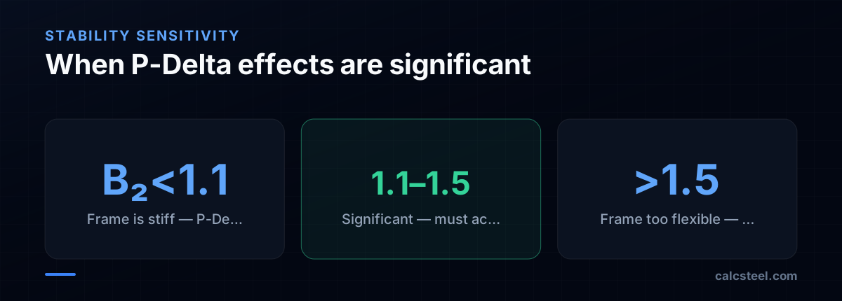
• B₂ < 1.10: Second-order effects are minor. A first-order analysis with B₁-B₂ amplification is adequate.
• 1.10 < B₂ < 1.50: Second-order effects are significant. A rigorous second-order analysis is recommended.
• B₂ > 1.50: The frame is too flexible. Redesign is needed — add bracing or increase member sizes.
• B₂ > 2.50: AISC does not permit this. The frame is approaching instability.

What makes B₂ large?

1. Heavy gravity loads (many stories of floor load)
2. Flexible lateral system (moment frames, especially with long spans)
3. Tall stories (the drift increases with story height)
4. Few lateral-resisting bays (concentrated resistance)

For a typical 10-story moment frame: B₂ ≈ 1.15–1.30. For a 3-story braced frame: B₂ ≈ 1.02–1.05.

The B₁-B₂ method (AISC Appendix 8) is an approximate way to get second-order forces from a first-order analysis:

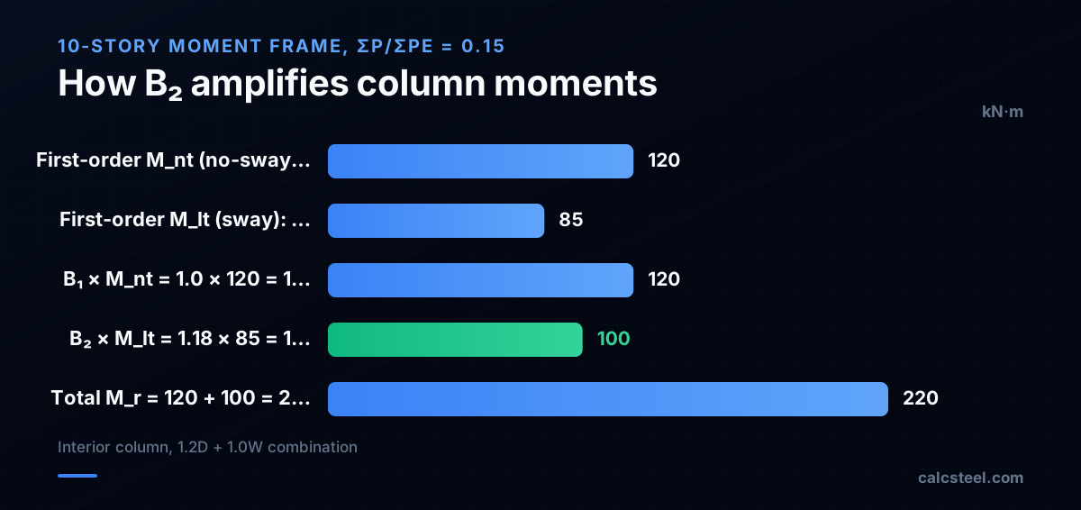
M_r = B₁ × M_nt + B₂ × M_lt

Where: - M_nt = moment from the "no-translation" (braced) analysis — all lateral displacement prevented - M_lt = moment from the "lateral-translation" analysis — only lateral loads with displacement - B₁ = non-sway amplifier = C_m / (1 − P_r/P_e1) ≥ 1.0 - B₂ = sway amplifier = 1 / (1 − ΣP_r/ΣP_e) ≥ 1.0

Step-by-step procedure

1. Run two first-order analyses: - Analysis 1 (nt): Apply all loads with a fictitious lateral support at each floor → get M_nt - Analysis 2 (lt): Apply only the lateral loads (wind, seismic, notional) without the fictitious supports → get M_lt

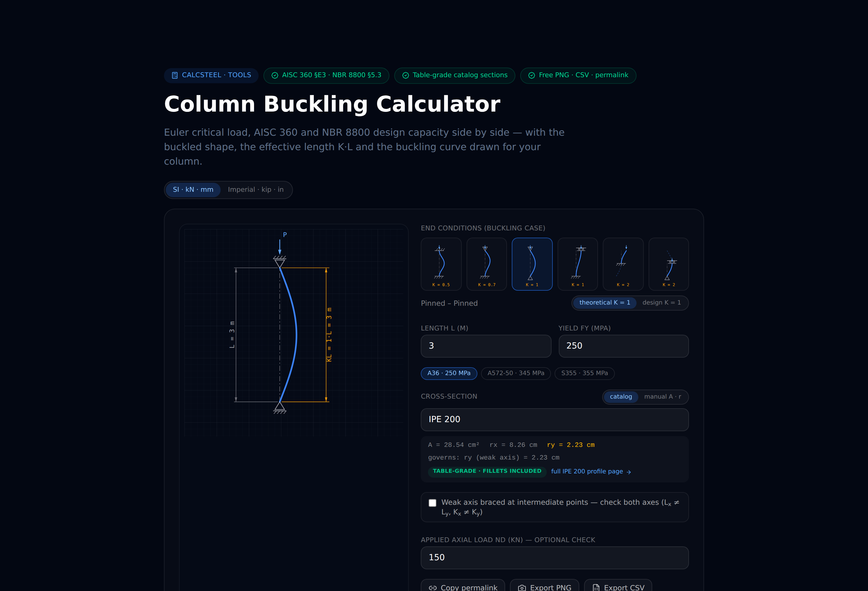
1. Calculate B₁ for each member: - C_m = 0.6 − 0.4(M₁/M₂) for members with end moments only (no transverse loads) - C_m = 1.0 for members with transverse loads between supports - P_e1 = π²EI/(K₁L)² where K₁ ≤ 1.0 (non-sway effective length) — you can size P_e for a single column with our free column buckling calculator (no sign-up needed)

1. Calculate B₂ for each story: - ΣP_r = total factored gravity load on the story - ΣP_e = Σπ²EI/(K₂L)² summed over all columns in the story - Alternatively: ΣP_e = R_M × ΣH × L / Δ_H where ΣH is the story shear and Δ_H is the first-order drift

1. Combine: M_r = B₁ × M_nt + B₂ × M_lt for each member

The Direct Analysis Method (DAM) is the preferred approach in AISC 360-22 because it avoids the B₁-B₂ decomposition and K-factor determination entirely.

DAM requirements

1. Notional loads: Apply 0.002 × Y_i as a lateral load at each level, where Y_i is the gravity load at that level. These represent initial out-of-plumbness.

1. Reduced stiffness: Use 0.8 × τ_b × EI for all members (flexure) and 0.8 × EA (axial), where: - τ_b = 1.0 when P_r/P_y ≤ 0.5 - τ_b = 4 × (P_r/P_y) × (1 − P_r/P_y) when P_r/P_y > 0.5

1. K = 1.0 for all members — No alignment charts, no sway/non-sway classification.

1. Second-order analysis: Run a rigorous second-order analysis (geometric nonlinear) on the modified model.

Why DAM works

By reducing the stiffness and adding notional loads, DAM captures: - Initial imperfections (out-of-plumb columns) - Residual stress effects (through τ_b) - Geometric nonlinearity (P-Δ and P-δ through the second-order analysis)

The result: the member forces from the analysis already include all second-order effects. No amplification factors are needed. K = 1.0 because the stability effects are accounted for in the analysis itself.

Advantages over B₁-B₂

• Eliminates K-factor subjectivity
• Handles leaning columns correctly
• Works for any frame geometry (not just regular frames)
• Gives one consistent set of forces for design

Second-order effects increase the internal forces in the frame. The impact varies by member type:

Columns (most affected)

• End moments increase by B₂ (typically 10–30% for moment frames)
• The interaction ratio (H1) increases because both P_r and M_r increase
• Columns in lower stories are most affected because they carry the highest ΣP
• Leaning columns transfer their P-Δ effect to the moment frame columns

Beams

• Beam end moments increase in moment frames (the beam shares the amplified moment with the column)
• Midspan moments are less affected (primarily a P-δ effect, which is small for beams)
• Beam shear at connections increases slightly

Connections

• Moment connections must be designed for the amplified end moments
• Simple shear connections are typically unaffected (they do not transfer moment)
• Base plate connections must resist the amplified column end moment

Bracing members

• Brace forces increase in proportion to the amplified story shear
• For stiff braced frames, the increase is small (B₂ ≈ 1.02–1.05)
• For eccentric braces, the link shear increases

Example impact

For a moment frame column with B₂ = 1.20: - First-order moment: 200 kN·m → second-order: 240 kN·m (+20%) - Interaction ratio: 0.75 → 0.88 (+17%) - The column still passes, but the margin drops from 25% to 12%

Ignoring P-Delta in this case would show a 25% margin that doesn't actually exist.

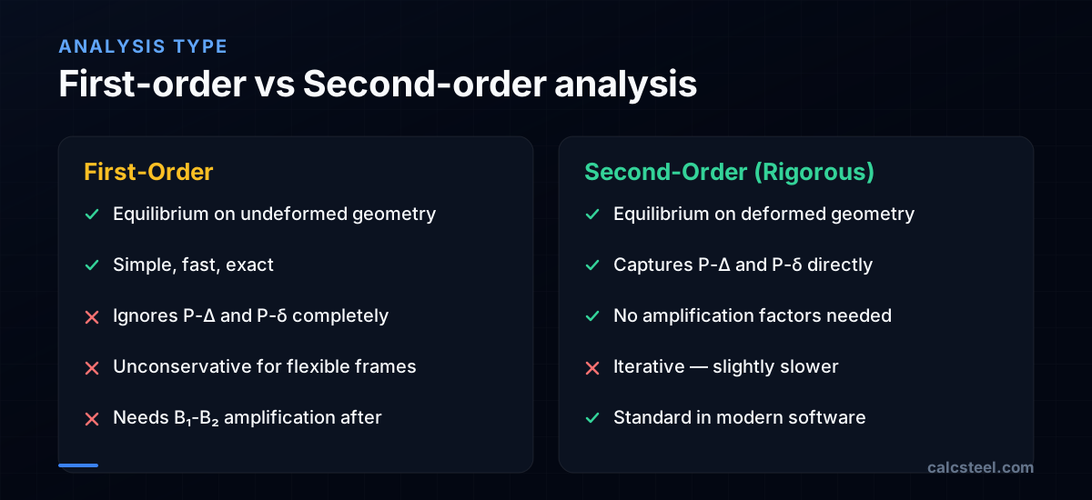
Geometric nonlinear analysis (GNA) is the rigorous way to capture P-Delta effects. Instead of amplifying first-order results, GNA solves equilibrium on the deformed geometry directly.

How GNA works

1. Apply all loads and solve the linear system → get displacements
2. Update the member geometry using the computed displacements
3. Re-form the stiffness matrix including geometric stiffness terms
4. Solve again on the updated geometry → get new displacements
5. Repeat until convergence (displacements stop changing)

Typically, 3–5 iterations are sufficient for most structures. If convergence is not reached, the structure is approaching instability (the loads exceed the elastic buckling capacity).

Geometric stiffness matrix

The key to GNA is the geometric stiffness matrix K_g, which modifies the elastic stiffness K_e:

[K_e + K_g] × {u} = {F}

For compression members, K_g is negative — it reduces the effective stiffness. This is the mathematical representation of P-Delta: compression makes the structure more flexible.

For tension members, K_g is positive — tension stabilizes the structure (like a guitar string getting stiffer when tightened).

When to use GNA vs B₁-B₂

• B₁-B₂: Adequate for simple frames, quick checks, hand calculations
• GNA: Required for complex frames, when B₂ > 1.10, or when using the Direct Analysis Method
• CalcSteel always uses GNA with the Direct Analysis Method as the default

1. Double-counting amplification

If your software runs a second-order analysis, the results already include P-Δ and P-δ effects. Applying B₁-B₂ on top of second-order results double-counts the amplification and is overly conservative.

2. Using first-order analysis for K-factor determination

K-factors from alignment charts assume first-order behavior. If you are using K > 1.0 for sway columns, you should be using first-order analysis + effective length method, NOT second-order analysis + K > 1.0. Mix and match creates inconsistencies.

3. Ignoring notional loads in DAM

The Direct Analysis Method requires notional loads (0.002Yi) to work correctly. Without them, the analysis does not capture initial imperfections, and the K = 1.0 simplification is not valid.

4. Forgetting that B₂ applies to the entire story

B₂ is a story-level quantity — it is the same for all columns in a given story. Computing B₂ per column is incorrect and gives non-equilibrium results.

5. Not checking convergence

A second-order analysis that does not converge indicates an unstable structure. Do not accept "last iteration" results as valid — the structure needs redesign.

6. Neglecting P-δ in individual members

Some software only captures P-Δ (story sway) but not P-δ (member curvature). For members with large axial loads and transverse loads between ends (e.g., columns with wind load), P-δ can be significant. Verify that your software accounts for both effects.

CalcSteel implements the full Direct Analysis Method with rigorous second-order analysis as the default:

Analysis method

• Geometric nonlinear analysis with P-Δ and P-δ effects
• Automatic convergence checking (typically 3–5 iterations)
• Notional loads applied automatically (0.002Yi at each level)
• Stiffness reduction (0.8τbEI and 0.8EA) applied to all members

K-factor handling

• K = 1.0 for all members (per DAM)
• No alignment charts needed
• No sway/non-sway classification required

Results

• All member forces include second-order amplification
• The B₂ sensitivity index is reported for each story
• If any story has B₂ > 1.5, a warning is issued
• Convergence status is shown in the analysis log

Stability check

The engine performs a global stability check by computing the elastic critical load factor (λ_cr = ΣP_e/ΣP_r). If λ_cr < 2.5, the structure may be too close to instability and a warning appears.

The combination of DAM + GNA gives the most reliable and consistent results for steel frame design. It handles regular and irregular frames, leaning columns, multi-story buildings, and any combination of lateral systems.