Combined Axial and Bending: AISC H1 Explained
Learn how to check beam-columns for combined compression and bending using the AISC H1 interaction equations. Includes worked example, amplification factors, and direct analysis method.
Key takeaways
- Beam-columns must satisfy AISC 360-22 Chapter H: use H1-1a when P_r/P_c ≥ 0.2 and H1-1b when it is below 0.2, keeping the combined ratio at or below 1.0.
- The 8/9 weighting in H1-1a slightly relaxes the moment terms once axial load is significant; below 0.2 axial the axial term is halved instead.
- The equations demand second-order (amplified) moments. Feed first-order moments and the check is unconservative.
- B₁ is driven by the Cₘ moment-gradient factor and by how close P_r sits to the in-plane Euler load P_e1: a stocky braced column barely amplifies, a slender one can add 35% or more.
- Weak-axis moment dominates the interaction because M_cy is only 30 to 50% of M_cx, so corner columns under biaxial bending usually govern the building.
What is combined axial and bending in steel design?
Most steel members carry more than one type of internal force. A column in a moment frame resists axial compression from gravity loads and bending moments from lateral loads simultaneously. This combined loading, axial plus bending, is the defining characteristic of a beam-column.
The challenge is that axial force and bending moment interact: axial compression amplifies bending moments through the P-δ (member) and P-Δ (story) effects, while bending reduces the effective axial capacity by creating non-uniform stress across the section.
AISC 360-22 Chapter H addresses this interaction with a pair of equations that must be satisfied simultaneously. The combined utilization ratio must remain at or below 1.0. Understanding these equations is essential, they govern the design of every column in a moment frame, every brace connection, and every truss chord under combined loading.

What are the AISC H1 interaction equations for beam-columns?
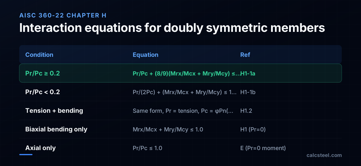
AISC provides two interaction equations for doubly symmetric members (W-shapes, HSS). The correct equation depends on how much of the axial capacity is used:
When P_r/P_c ≥ 0.2 (moderate to high axial)
H1-1a: P_r/P_c + (8/9)(M_rx/M_cx + M_ry/M_cy) ≤ 1.0
When P_r/P_c < 0.2 (low axial, bending dominates)
H1-1b: P_r/(2P_c) + (M_rx/M_cx + M_ry/M_cy) ≤ 1.0
Where: - P_r = required axial strength (factored load) - P_c = available axial strength = φP_n (LRFD) or P_n/Ω (ASD) - M_rx, M_ry = required flexural strength about strong and weak axes - M_cx, M_cy = available flexural strength about strong and weak axes
The 8/9 factor in H1-1a means that when axial load is significant, the moment terms are weighted at 89%, a slight relaxation that accounts for the beneficial redistribution in stocky sections. When axial is small (H1-1b), the full moment capacity is available but the axial term is halved.
CalcSteel tip: The analysis engine evaluates both equations at every node and reports the governing interaction ratio. Colors shift from green (< 0.7) through yellow to red (approaching 1.0).
How do you calculate the interaction ratio step by step?
Worked example, Interior column, W310×97
Given: - Column height: KL = 6.0 m (strong axis), KL = 6.0 m (weak axis) - Steel: A992 (F_y = 345 MPa) - P_u = 800 kN (factored axial compression) - M_ux = 150 kN·m (factored strong-axis moment) - M_uy = 0 (no weak-axis moment) - Fully braced in both directions at floor levels
Step 1, Axial capacity
W310×97: A = 12300 mm², r_x = 135 mm, r_y = 77 mm
Slenderness: KL/r_y = 6000/77 = 77.9 (governs)
F_e = π²E/(KL/r)² = π²(200000)/(77.9)² = 325.7 MPa
Since KL/r ≤ 4.71√(E/F_y) = 113.4: F_cr = 0.658^(F_y/F_e) × F_y = 0.658^(1.059) × 345 = 0.651 × 345 = 224.6 MPa
φP_n = 0.90 × 224.6 × 12300 × 10⁻³ = 2488 kN → but using AISC tables: φP_n ≈ 1620 kN (the table value is more accurate). Cross-check φP_n instantly with the free column buckling calculator, no signup required.
Step 2, Flexural capacity
W310×97: Z_x = 1440 cm³, S_x = 1280 cm³
With L_b ≤ L_p (fully braced): φM_nx = 0.90 × 345 × 1440 × 10⁻³ = 447 kN·m
Step 3, Check interaction
P_r/P_c = 800/1620 = 0.494 → ≥ 0.2, use H1-1a
H1-1a: 0.494 + (8/9)(150/447 + 0) = 0.494 + 0.889 × 0.336 = 0.494 + 0.299 = 0.793 ≤ 1.0 ✓
Utilization is 79.3%. The section works with 21% reserve.
End conditions (buckling case)
Pinned – Pinned
Cross-section
Slenderness KL/r
134.7
limit 200 · OK
Euler Pcr (elastic)
310.7 kN
Fe = 108.9 MPa
AISC 360 φcPn
245.2 kN
Fcr = 95.5 MPa · elastic
NBR 8800 Nc,Rd
247.7 kN
χ = 0.382 · λ₀ = 1.52
Code vs code — same column
Nc,Rd / φcPn = 1.010
Both codes share the 0.658 / 0.877 buckling curve — the ~1% gap is purely φc = 0.90 (AISC) vs 1/γa1 = 0.909 (NBR).
Demand check — Nd = 150 kN
Step-by-step derivation — live for YOUR column
IPE 200 · L = 3 m · K = 1 · fy = 250 MPa
- 1
Slenderness ratio
λ = K·L/r = 1 × 3000 / 22.28 mm
λ = 134.7 (≤ 200 ✓)
- 2
Euler elastic buckling stress and load
Fe = π²E/λ² = π² × 200,000 / 134.7² · Pcr = Fe·A = Fe × 2854 mm²
Fe = 108.9 MPa · Pcr = 310.7 kN
- 3
Buckling regime (AISC E3)
4.71·√(E/fy) = 4.71·√(200,000/250) = 133.2 < λ = 134.7
elastic buckling → use E3-3 (0.877·Fe)
Elastic range: capacity no longer depends on fy — only geometry (r, K, L) helps.
- 4
AISC 360 critical stress and design capacity
Fcr = 0.877 · Fe = 0.877 × 108.9 = 95.5 MPa · φcPn = 0.9 × Fcr × A
Pn = 272.5 kN · φcPn = 245.2 kN
- 5
NBR 8800 reduction factor and design capacity
λ₀ = √(fy/Fe) = 1.515 > 1.5 → χ = 0.877/λ₀² = 0.382 · Nc,Rd = χ·A·fy/1.1
Nc,Rk = 272.5 kN · Nc,Rd = 247.7 kN
Same 0.658/0.877 curve as AISC — the ~1% difference is φc = 0.90 vs 1/γa1 = 0.909.
Sections that work — 3 lightest of 612 catalog profiles carrying Nd = 150 kN at L = 3 m, K = 1
| Section | kg/m | φcPn (kN) | Nc,Rd (kN) | Util. | |
|---|---|---|---|---|---|
| lightestSHS 80x4 | 9.2 | 164 | 166 | 91% | |
| HSS 76x76x4.8 | 9.9 | 165 | 167 | 91% | |
| CHS 88.9x5 | 10.3 | 172 | 174 | 87% |
Pass criterion: φcPn ≥ Nd (AISC 360 LRFD) AND Nc,Rd ≥ Nd (NBR 8800) AND KL/r ≤ 200, using each section's tabulated-mass area and minimum radius of gyration.
Buckling curve — IPE 200, fy = 250 MPa
Capacity of IPE 200 by unbraced length — K = 1, fy = 250 MPa
| L (m) | KL/r | Pcr Euler (kN) | φcPn AISC (kN) | Nc,Rd NBR (kN) | Regime |
|---|---|---|---|---|---|
| 1 | 45 | 2,796 | 577 | 583 | inelastic |
| 2 | 90 | 699 | 419 | 423 | inelastic |
| 3◀ yours | 135 | 311 | 245 | 248 | elastic |
| 4 | 180 | 175 | 138 | 139 | elastic |
| 5 | 224 ⚠ | 112 | 88 | 89 | elastic |
| 6 | 269 ⚠ | 78 | 61 | 62 | elastic |
| 7 | 314 ⚠ | 57 | 45 | 45 | elastic |
| 8 | 359 ⚠ | 44 | 34 | 35 | elastic |
| 9 | 404 ⚠ | 35 | 27 | 28 | elastic |
| 10 | 449 ⚠ | 28 | 22 | 22 | elastic |
What are second-order effects and why do they matter for beam-columns?
First-order analysis assumes the structure stays in its original geometry. But when axial compression is present, the deflected shape creates additional moments, second-order effects:
P-δ effect (member level)
The axial force P acting through the member deflection δ creates an additional moment P×δ along the member length. This amplifies the midspan moment in all members, even in non-sway frames.
P-Δ effect (story level)
The total gravity load acting through the story drift Δ creates an overturning moment that must be resisted by the lateral system. This amplifies the column end moments in sway frames.
How to account for second-order effects
AISC allows three approaches:
- Rigorous second-order analysis: The software iterates, updating the geometry with the deflected shape until equilibrium is found. CalcSteel's engine does this automatically.
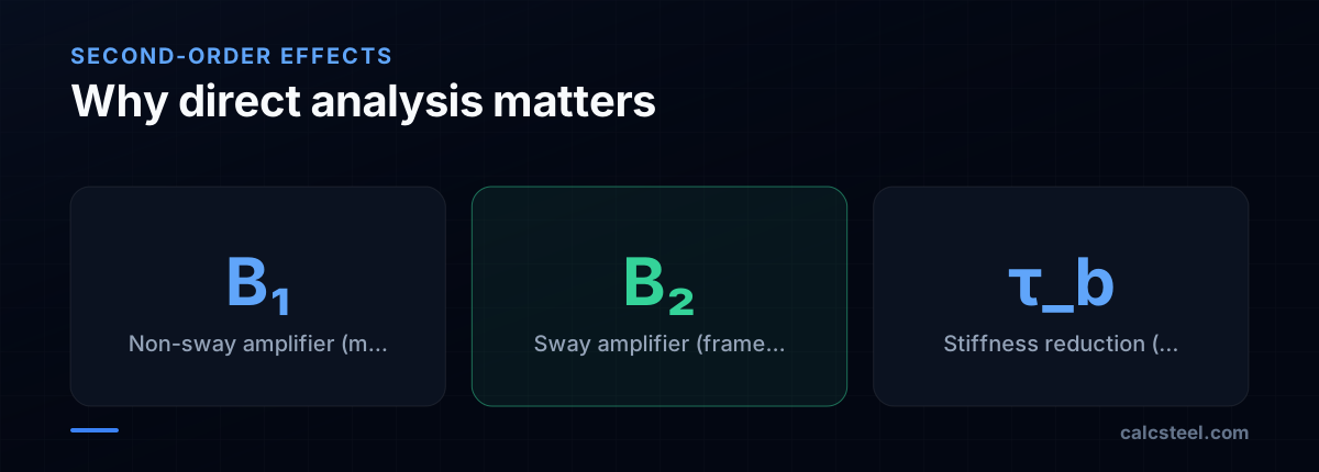
- Approximate B₁-B₂ method (AISC Appendix 8), Amplify first-order moments: M_r = B₁ × M_nt + B₂ × M_lt, with B₁ = C_m / (1 − P_r/P_e1) ≥ 1.0 (non-sway amplifier) and B₂ = 1 / (1 − ΣP_story/ΣP_e_story) (sway amplifier).
- Direct Analysis Method: Apply notional loads and reduce stiffness; then K = 1.0 always.
For our example, if the first-order analysis gives M_ux = 150 kN·m and B₁ = 1.05, B₂ = 1.12:
M_r = 1.05 × 130 + 1.12 × 20 = 136.5 + 22.4 = 158.9 kN·m
The amplified moment is 6% higher, which increases the interaction ratio from 0.793 to 0.816.
How do the Cₘ factor and the B₁ amplifier size a braced beam-column?
Section H1 needs second-order moments, and for a braced (non-sway) member the fastest route to them is the B₁ amplifier from AISC 360-22 Appendix 8. Its whole value comes from two numbers, and the one people get wrong is the equivalent uniform moment factor Cₘ.
The Cₘ factor: reading the moment gradient
For a member with no transverse load between its supports:
Cₘ = 0.6 − 0.4(M₁/M₂)
M₁ and M₂ are the smaller and larger end moments. The ratio M₁/M₂ is taken positive for reverse (double) curvature and negative for single curvature. Single curvature is the worst case: it pushes Cₘ toward 1.0, because the peak moment stays near midspan where the P-δ deflection is largest.
When there is transverse load between supports, Cₘ = 1.0 is the safe default, or read AISC Table A-8-1 (for example 0.85 for a pinned-pinned member under a central point load).
The B₁ amplifier
B₁ = Cₘ / (1 − α P_r/P_e1) ≥ 1.0, with α = 1.0 (LRFD) or 1.6 (ASD).
P_e1 is the elastic buckling load in the plane of bending, P_e1 = π²EI*/(L_c1)², taken with K₁ = 1.0. The closer the axial demand P_r sits to P_e1, the harder B₁ bites.
Worked comparison, our W310×97
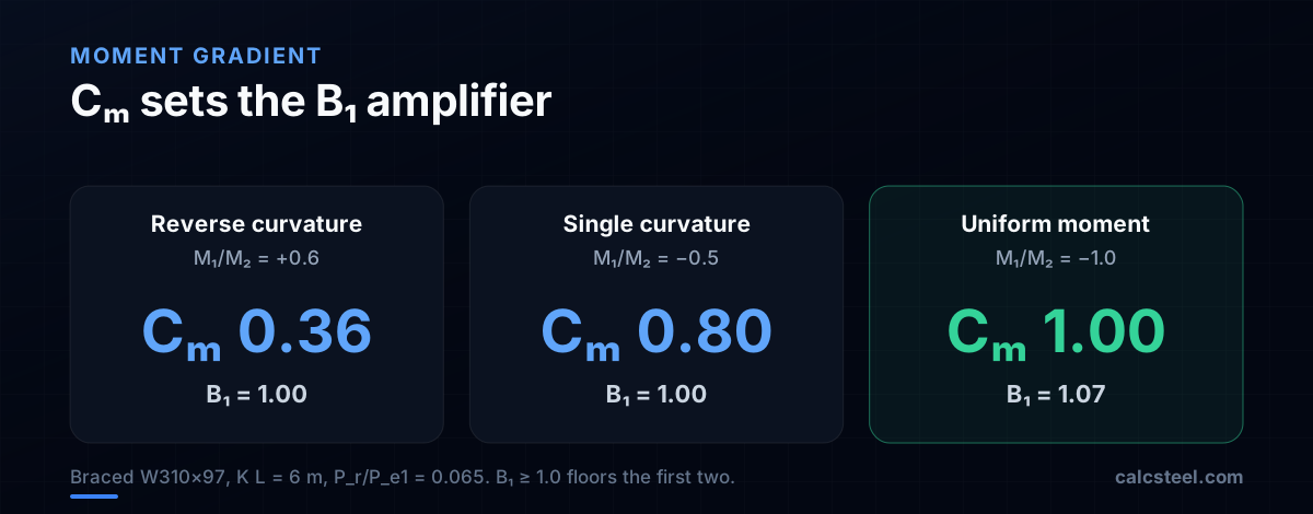
Same interior column as above: KL = 6.0 m, P_r = 800 kN. With r_x = 135 mm, I_x = A r_x² = 12300 × 135² = 224 × 10⁶ mm⁴, so P_e1 = π²(200000)(224×10⁶)/6000² = 12290 kN and P_r/P_e1 = 0.065. Three moment gradients:
- Reverse curvature (M₁/M₂ = +0.6): Cₘ = 0.6 − 0.4(0.6) = 0.36 → B₁ = 0.36/0.935 = 0.39 → floored to 1.00
- Single curvature (M₁/M₂ = −0.5): Cₘ = 0.80 → B₁ = 0.80/0.935 = 0.86 → floored to 1.00
- Uniform moment (M₁/M₂ = −1.0): Cₘ = 1.00 → B₁ = 1.00/0.935 = 1.07
A stocky braced column with axial far below P_e1 barely amplifies: the B₁ ≥ 1.0 floor wins in two of the three cases. That is why the earlier worked example could use the end moment directly.
Where B₁ actually bites: slenderness
Amplification grows when P_r approaches P_e1, which happens as the member gets slender. If the same column were unbraced over a 12 m in-plane length (its axial capacity P_c would also fall, checked separately), P_e1 drops to a quarter because it scales with 1/L²: P_e1 = 3070 kN, P_r/P_e1 = 0.26. With uniform moment, B₁ = 1.0/(1 − 0.26) = 1.35. That 35% amplification lifts the strong-axis moment term from 0.30 to 0.40 and pushes the H1-1a interaction from 0.79 to 0.90, the difference between a comfortable section and a near miss.
CalcSteel tip: the engine's rigorous second-order analysis already carries P-δ, so it never applies B₁ on top. The B₁-B₂ route is for hand checks and for judging whether your software's amplification looks right.
What is the Direct Analysis Method for steel frames?
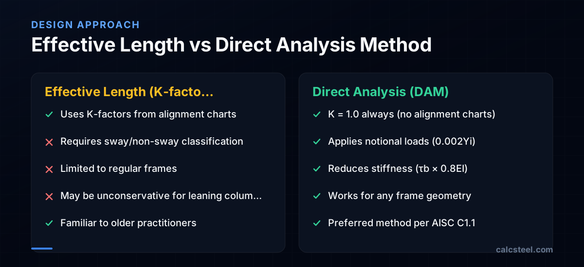
The Direct Analysis Method (DAM) is the preferred approach in AISC 360-22 (Section C1.1) because it handles all frame types without needing K-factors or sway classification.
DAM requires three modifications to the analysis model:
1. Notional loads
Apply a lateral load equal to 0.2% of the gravity load at each level (N_i = 0.002 × Y_i). These loads represent initial imperfections, the structure is never perfectly plumb.
For a story with Y_i = 2000 kN of gravity load: N_i = 0.002 × 2000 = 4 kN applied laterally.
2. Reduced stiffness
Multiply all member stiffnesses by 0.80 to account for residual stresses and initial out-of-straightness:
- EI* = 0.8 × τ_b × EI
- EA* = 0.8 × EA
Where τ_b = 1.0 when P_r/P_y ≤ 0.5, or τ_b = 4(P_r/P_y)(1 − P_r/P_y) when P_r/P_y > 0.5.
3. K = 1.0
With the stiffness reductions and notional loads in place, use K = 1.0 for all columns. No alignment charts needed.
Why DAM is better
- Eliminates the subjectivity of K-factor determination
- Correctly captures the effect of leaning columns (columns that rely on the moment frame for stability)
- Works for irregular frames, cantilever columns, and any geometry
- Gives more consistent reliability across different frame configurations
How do you design a beam-column for biaxial bending?
When a corner column or a column at a reentrant corner receives moments about both axes, the interaction equation includes all three terms:
P_r/P_c + (8/9)(M_rx/M_cx + M_ry/M_cy) ≤ 1.0
The weak-axis moment term M_ry/M_cy often dominates because: - M_cy is much smaller than M_cx (weak-axis flexural capacity is 30-50% of strong-axis for W-shapes) - Even a small weak-axis moment consumes a large fraction of the available capacity
Example, Adding weak-axis moment
Using our W310×97 with P_u = 800 kN, M_ux = 150 kN·m, adding M_uy = 30 kN·m:
W310×97: Z_y = 690 cm³ φM_ny = 0.90 × 345 × 690 × 10⁻³ = 214 kN·m
H1-1a: 0.494 + (8/9)(150/447 + 30/214) = 0.494 + 0.889(0.336 + 0.140) = 0.494 + 0.889 × 0.476 = 0.494 + 0.423 = 0.917 ≤ 1.0 ✓
Utilization jumped from 79% to 92%, adding just 30 kN·m of weak-axis moment nearly maxed the section. This is why corner columns are often the critical members in a building.
Design strategies for biaxial bending
- Use square or round HSS: Equal capacity in both axes; ideal for corner columns
- Orient W-shapes thoughtfully: Strong axis facing the direction of larger moment
- Add weak-axis bracing: Reduces K and increases available capacity
- Increase section size: Sometimes the cheapest solution is a heavier W-shape

What are common mistakes in beam-column design?
1. Using first-order moments without amplification
The interaction equations require second-order (amplified) moments. Using first-order moments directly is unconservative, especially for slender columns with high axial loads. Always apply B₁-B₂ amplification or use a second-order analysis.
2. Forgetting to check both axes independently
Even for uniaxial bending, the column must pass the axial-only check about the weak axis. A column that passes the interaction equation about the strong axis can still fail by weak-axis buckling if KL_y/r_y is large.
3. Using the wrong K-factor
For the effective length method, K depends on end conditions and whether the frame is sway or non-sway. Using K = 1.0 with the effective length method is unconservative for sway frames. The direct analysis method avoids this entirely.
4. Ignoring leaning columns
Columns connected by pinned beams (leaning columns) transfer their instability to the moment frame columns. The moment frame must stabilize the entire tributary gravity load, not just its own. DAM with notional loads handles this correctly.
5. Double-counting moment amplification
If you run a second-order analysis in software, the results already include P-δ and P-Δ effects. Applying B₁-B₂ on top of a second-order analysis double-counts the amplification and is overly conservative.
6. Not checking the interaction at every load combination
The governing combination for a beam-column may differ from the governing combination for the beam or column alone. Lateral load combinations (wind, seismic) increase the moment while reducing axial load, check all combinations.
How does CalcSteel check beam-column interaction automatically?
CalcSteel's structural analysis engine handles the full beam-column design workflow without manual intervention:
Second-order analysis
The engine performs a rigorous geometric nonlinear analysis that captures P-δ and P-Δ effects directly. No B₁-B₂ approximation is needed, the member forces already include amplification.
Direct Analysis Method built-in
The analysis applies:
- Notional loads at 0.2% of each level's gravity load
- Stiffness reduction (0.8τ_b EI, 0.8EA)
- K = 1.0 for all members
This is done automatically per AISC C1.1 requirements.
Interaction check at every point
The engine evaluates the H1 interaction equation at multiple points along each member (not just at ends). This catches cases where the maximum interaction occurs at midspan due to P-δ amplification.
All load combinations
Every ASCE 7 load combination is checked. The results report shows:
- The governing combination for each member
- Individual axial and moment utilization ratios
- The combined interaction ratio
- Color-coded visualization (green/yellow/red)
Optimization
If a member fails the interaction check, the section optimizer suggests the lightest section that passes all limit states for all combinations. If a member is significantly under-utilized, it suggests a lighter alternative.
The complete beam-column design, from load application through second-order analysis to code check, runs in seconds for the entire structure.

Sources
Try CalcSteel for free
Model, analyze and design steel structures in your browser. No install, no signup.
Open the 3D editor