Effective Length Factor K in Column Design

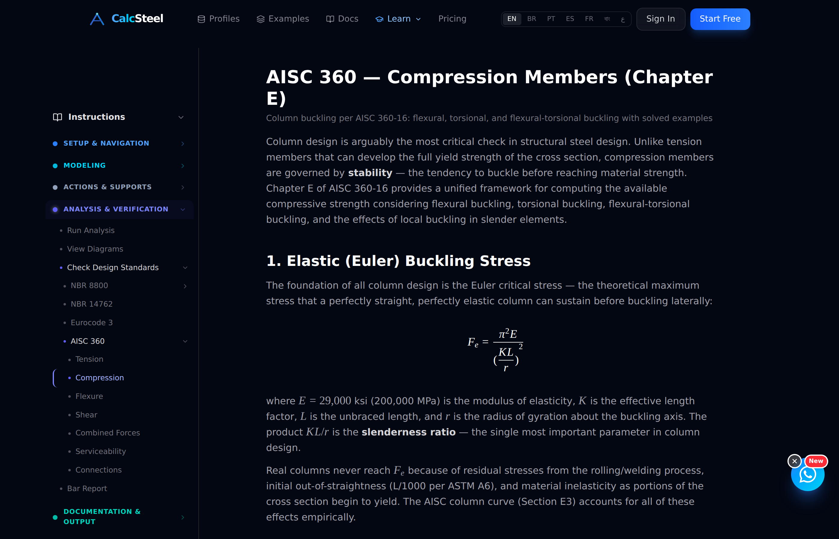
In 1744 Leonhard Euler solved the buckling of an ideal, pin-ended column and found that the critical load is P_cr = π²EI / L². The formula assumes both ends can rotate freely but cannot translate. That is one specific boundary condition — and in real buildings, columns almost never look like that.

The effective length factor K is a multiplier that converts the actual unbraced length L into an equivalent length KL of a pin-ended column with the same critical load. Fixed ends shorten the buckling wave (K < 1), while a free top (cantilever) doubles it (K = 2). The slenderness ratio the code actually uses is KL/r, not L/r.

Every modern steel design standard — AISC 360, NBR 8800, Eurocode 3, IS 800 — builds its compression-capacity curve on this same idea. The column’s strength starts at the yield load (short, stocky columns) and drops along the Euler hyperbola as KL/r increases. Getting K right is therefore the single most leveraged input in column design: everything downstream — F_cr, φP_n, the profile you pick, the steel you buy — depends on it.

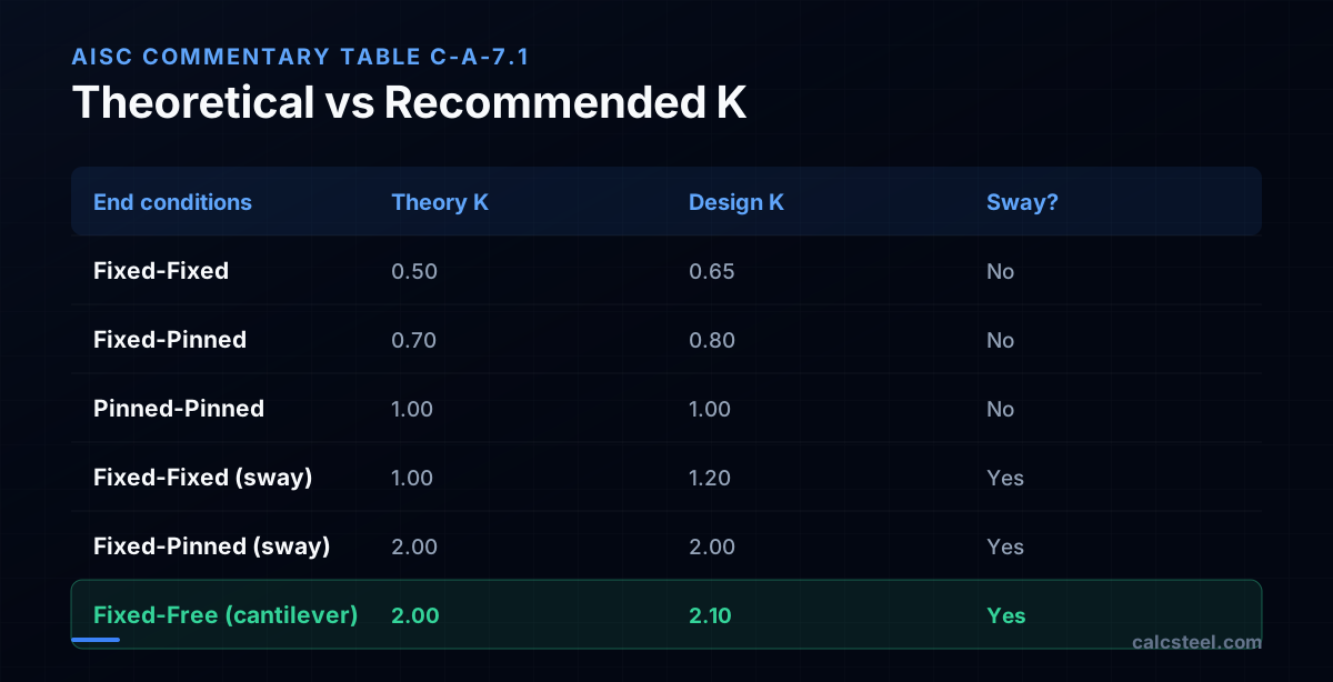
AISC 360 Commentary Table C-A-7.1 (and NBR 8800 Annex H) list six idealised cases. Two numbers appear for each: the theoretical K from an exact stability solution, and the recommended design K, which is always larger because real connections are never infinitely stiff.

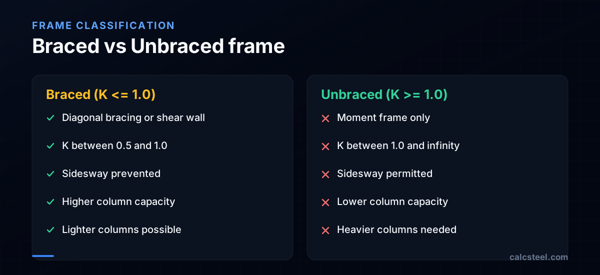
The table below summarises all six cases. Three belong to braced frames (sidesway prevented, K ≤ 1.0) and three to unbraced frames (sidesway permitted, K ≥ 1.0):

• Fixed–Fixed, braced: Theory K = 0.50, design K = 0.65. The column buckles in a full S-curve with two inflection points; the effective length is barely half the physical length.
• Fixed–Pinned, braced: Theory K = 0.70, design K = 0.80. One end rotates; the inflection point is roughly 30% from the pinned end.
• Pinned–Pinned, braced: K = 1.00 in both theory and design — this is Euler’s original case, the baseline.
• Fixed–Fixed, sway: Theory K = 1.00, design K = 1.20. Both ends are rotationally fixed, but the top can translate laterally.
• Fixed–Pinned, sway: Theory K = 2.00, design K = 2.00. A flagpole with rotational restraint at the base only.
• Fixed–Free (cantilever): Theory K = 2.00, design K = 2.10. The worst case — the column buckles as a quarter-wave, and the effective length is more than double the physical length.

The gap between theory and design K is largest at the stiff end (0.50 → 0.65, a 30% bump) because “perfectly fixed” is a fiction: base plates have finite rotational stiffness, and beam-to-column connections always allow some rotation.

The theoretical K assumes mathematically perfect boundary conditions: infinite rotational stiffness at a ‘fixed’ end, zero stiffness at a ‘pinned’ end, and zero initial imperfections in the column. None of these are true in practice.

A bolted base plate on a concrete footing is never infinitely rigid — it has a finite rotational stiffness that depends on plate thickness, anchor bolt layout, grout, and even soil stiffness. A beam-to-column moment connection (end-plate, flange-welded) also allows some rotation under load. If you used K = 0.50 for a ‘fixed–fixed’ column and the real connection only delivers 80% of full fixity, the actual K might be closer to 0.58 — and your capacity would be overestimated by about 15%.

The recommended values absorb this uncertainty. AISC’s 0.65 for the fixed–fixed case essentially says: we trust your connection is mostly fixed, but we are not betting the building on it being perfect. This philosophy is echoed by NBR 8800, which uses the same recommended values in its Annex H, and by Eurocode 3 Part 1-1, which defines buckling lengths in terms of system-level elastic critical load analysis rather than isolated K values.

For the pinned–pinned case, theory and design agree at K = 1.00 because a simple shear connection (clip angles, shear tab) genuinely provides near-zero moment restraint — the idealisation matches reality.

This is where a single number makes or breaks a design. Let us take a concrete example: a W200x46 (A = 5 890 mm², r_y = 51.3 mm) made of A572 Gr. 50 steel (F_y = 345 MPa), with an unbraced length of 4 m. We check weak-axis flexural buckling per AISC 360-22 LRFD.

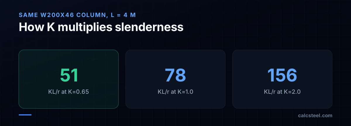
At K = 0.65 (fixed–fixed, braced): KL/r = 0.65 × 4 000 / 51.3 = 50.7. The Euler stress F_e = π²E/(KL/r)² = 768 MPa. Since F_e > 0.44F_y, AISC uses the inelastic curve: F_cr = 0.658^(F_y/F_e) × F_y = 286 MPa. Design capacity φP_n = 0.9 × 286 × 5 890 / 1 000 ≈ 1 520 kN.

At K = 1.00 (pinned–pinned): KL/r = 78.0, F_e = 324 MPa, F_cr = 221 MPa, φP_n ≈ 1 170 kN. Capacity drops 23%.

At K = 2.00 (cantilever): KL/r = 156, F_e = 81 MPa. Now KL/r exceeds 4.71√(E/F_y) = 113.4, so AISC switches to the elastic curve: F_cr = 0.877 × F_e = 71 MPa. φP_n ≈ 380 kN — a quarter of the fixed–fixed capacity.

The bar chart summarises all five cases. The takeaway: for this real-world column, the difference between the best and worst boundary condition is a factor of 4×. No other single input — steel grade, profile size, or even unbraced length — has this much leverage at constant geometry.

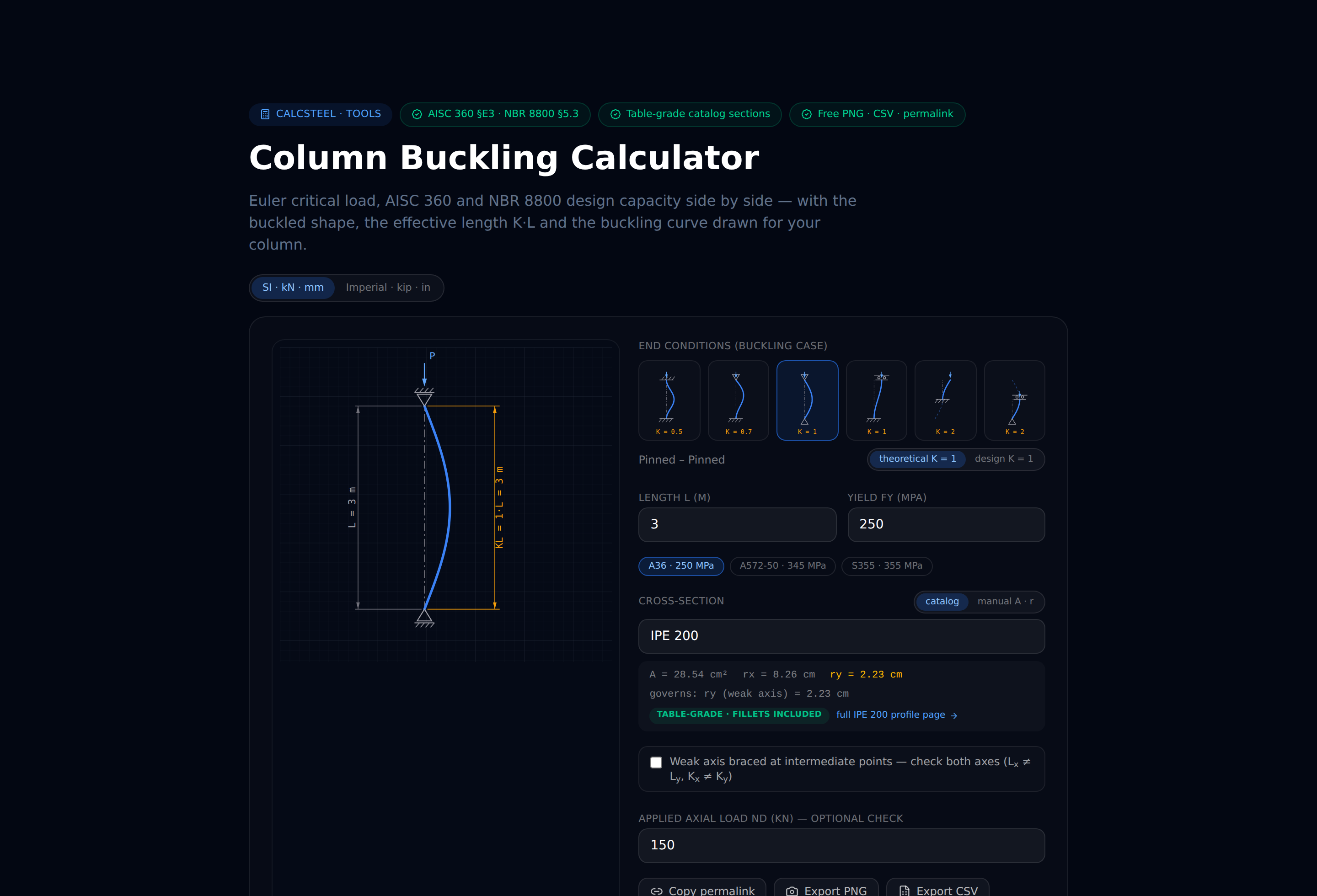
Want to try it on your own column? The free column buckling calculator runs this exact AISC 360 check in your browser — set K, length and profile, and read φP_n instantly, no signup.

The single most important classification for picking K is whether your frame is braced (sidesway inhibited) or unbraced (sidesway uninhibited). This distinction determines which half of the K table — and which alignment chart — applies.

A frame is braced when lateral displacement of the column top relative to the bottom is prevented by a separate lateral-force-resisting system: diagonal braces, concrete shear walls, or a diaphragm. In a braced frame, K is always ≤ 1.0, and the column can only buckle by bowing between its supports (no side-sway component).

A frame is unbraced (also called a moment frame or sway frame) when the columns and beams alone resist lateral loads through their bending stiffness. Here K is always ≥ 1.0, and the column can buckle in a sway mode — the entire storey drifts sideways. This dramatically reduces capacity.

AISC 360 Chapter C now offers the Direct Analysis Method (DAM) as the preferred approach for stability, which allows you to use K = 1.0 for all columns in the analysis model — but only if you include notional loads and reduced stiffness (τ_b × EI). The DAM captures the P-Delta effect directly in the analysis rather than through an inflated K. CalcSteel supports both approaches: you can set explicit K values per axis, or let the analysis capture second-order effects and use K = 1.0.

The six cases in the table above are idealisations: perfectly fixed or perfectly pinned ends. A real column sits between beams of finite stiffness, so its ends are partially restrained, somewhere between a pin and a fix. For that continuum, engineers use the alignment chart (also called the nomograph, after Jackson and Moreland), reproduced in the AISC 360 Commentary and in NBR 8800 Annex H. It turns the stiffness of the members framing into each end of the column into a value of K.

The input is a stiffness ratio G evaluated at each end of the column: G = Σ(EI/L)_columns / Σ(EI/L)_beams, the sum of the stiffnesses of the columns meeting at the joint divided by the sum of the stiffnesses of the beams (girders) framing into it, all taken in the plane of buckling. For members of the same steel grade E cancels, so G = Σ(I_c/L_c) / Σ(I_g/L_g). A small G means stiff beams relative to the column, so the joint is nearly fixed and K is low; a large G means flexible beams that let the joint rotate, so K climbs.

The two ends that frame into no beams need a convention. The AISC Commentary recommends G = 10 for a nominally pinned support (theoretically infinite) and G = 1.0 for a nominally fixed support (theoretically zero), for the same reason the recommended K values are higher than the theoretical ones: a real base is never a perfect hinge or a perfect clamp.

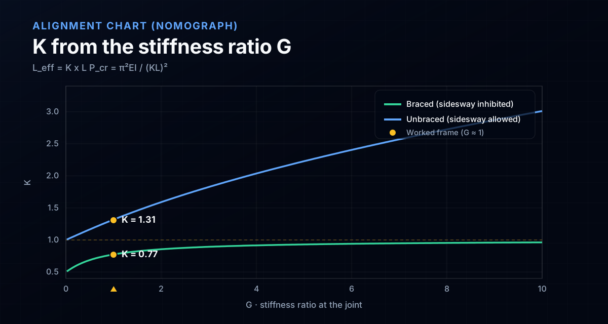
There are two charts, one for each side of the braced / unbraced split. Each is the graphical solution of a transcendental equation (AISC Commentary Equations C-A-7-1 and C-A-7-2):

• Braced (sidesway inhibited), K ≤ 1.0: (G_AG_B/4)(π/K)² + [(G_A+G_B)/2]·[1 − (π/K)/tan(π/K)] + (2/(π/K))·tan(π/2K) = 1.
• Unbraced (sidesway uninhibited), K ≥ 1.0: [G_AG_B(π/K)² − 36] / [6(G_A+G_B)] = (π/K)/tan(π/K).

On the printed nomograph you lay a straightedge across the G_A and G_B scales and read K where it crosses the middle scale. The chart below plots the same result for the symmetric case G_A = G_B: the braced curve stays between 0.5 and 1.0, while the sway curve starts at 1.0 and climbs without bound as the beams get weaker.

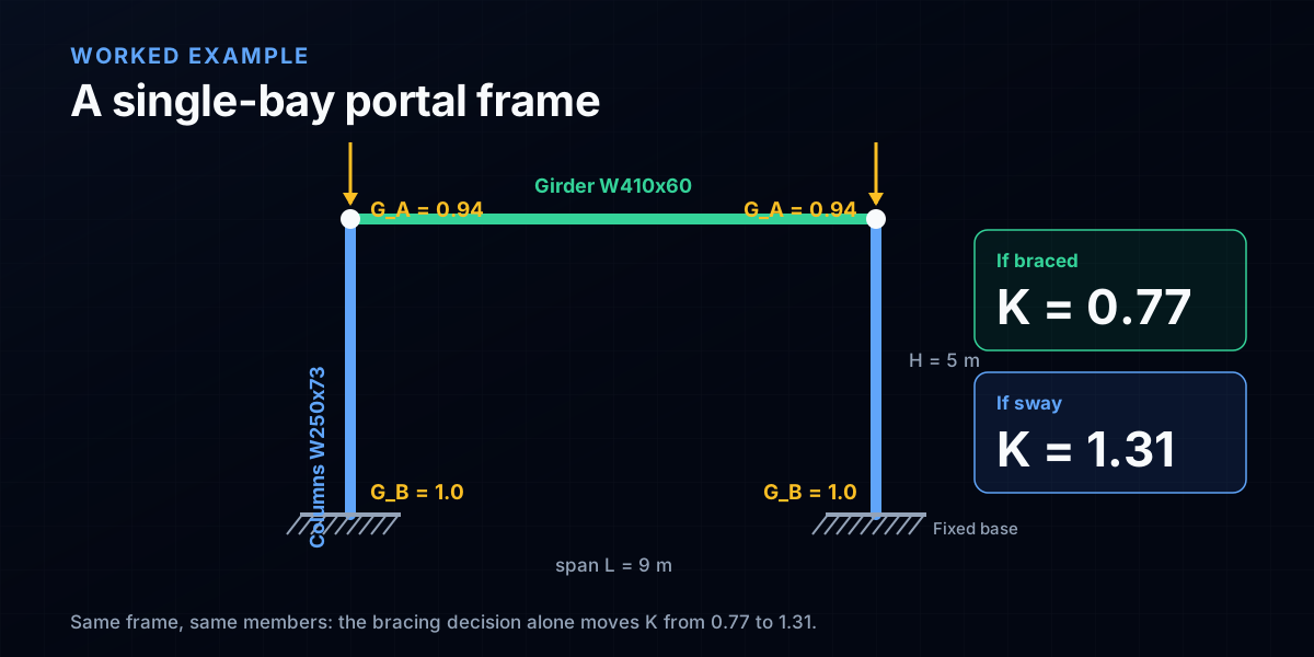
Take a single-bay portal frame: two W250x73 columns 5 m tall carrying a W410x60 girder over a 9 m span, with the column bases cast into the foundations and rigid (moment) connections at the top. From CalcSteel’s profile database the strong-axis second moments of area are I_c = 111 × 10⁶ mm⁴ for the column and I_g = 213 × 10⁶ mm⁴ for the girder.

Step 1: G at the top joint. One column and one girder meet there, both bending in the plane of the frame: G_A = (I_c/H) / (I_g/L) = (111 × 10⁶ / 5 000) / (213 × 10⁶ / 9 000) = 22 200 / 23 700 = 0.94.

Step 2: G at the base. The base is fixed, so G_B = 1.0, the AISC design recommendation for a fixed support.

Step 3: Pick the chart. If a separate bracing system (diagonals, a shear wall) carries the lateral load, use the braced chart. If the frame resists lateral load by bending of its own members, use the sway chart.

Step 4: Read K. Solving the two equations with G_A = 0.94 and G_B = 1.0 gives K = 0.77 braced and K = 1.31 unbraced (sway).

Same frame, same members, same G values: the single decision of whether the frame is braced moves K from 0.77 to 1.31. Because the Euler term scales as 1/K², the elastic buckling stress of that column in the sway frame is only (0.77/1.31)² ≈ 35% of its braced value. That is the whole reason the Direct Analysis Method exists: instead of chasing K up the alignment chart for every sway column, you capture the sidesway in the analysis itself and design with K = 1.0. Whichever route you take, CalcSteel lets you set K_x and K_y per member and reads the resulting capacity straight into the verification panel.

CalcSteel shows the effective length factor in two places: the design verification panel (per-member, with Kx and Ky) and the buckling diagrams documentation (the theory behind the numbers).

To set K for a column: select the member, open the Properties panel, and look for the Effective length fields. You will see separate Kx (strong axis) and Ky (weak axis) inputs. By default both are 1.0 — the pin–pin assumption. Change them to match your actual boundary conditions:

• Kx = Ky = 0.65 if both ends are moment-connected (flange welds or end-plates) and the frame is braced.
• Ky = 1.0, Kx = 1.2 if the column is braced against weak-axis buckling by a floor slab or girt, but sits in an unbraced moment frame in the strong direction.
• Kx = Ky = 2.0 for a true cantilever (fixed base, free top) — rare in buildings, common in signposts and light poles.

After you change K, re-run the analysis and open the Design Verification results. The utilisation ratio (demand/capacity) updates instantly. You can toggle K values and watch the ratio jump — this is the fastest way to build intuition for how K governs your design.

The screenshot below shows CalcSteel’s buckling reference page, which explains each K case with interactive diagrams. The full Buckling Diagrams article in the documentation section provides the underlying theory with Euler’s formula and all six classical cases.

After reviewing hundreds of student projects and forum posts (Reddit’s r/StructuralEngineering is a goldmine), these are the K-related mistakes that keep appearing:

1. Using K = 1.0 everywhere ‘to be conservative.’ This is safe for braced frames (K ≤ 1.0 by definition), but it is the opposite of conservative for unbraced frames where K should be 1.2 or higher. If your moment frame has no bracing and you used K = 1.0, you overestimated every column’s capacity.
2. Assuming a connection is ‘fixed’ without checking. A shear tab or clip-angle connection provides near-zero moment resistance — it is a pin, not a fix. Only connections explicitly designed for moment transfer (end-plates, directly welded flanges) justify K < 1.0. Even then, the recommended K = 0.65 (not 0.50) accounts for the connection being less than perfectly rigid.
3. Forgetting that Kx ≠ Ky. Strong-axis and weak-axis buckling have different unbraced lengths and different end restraints. A column braced at mid-height by a girt has Ky effectively halved (smaller K or smaller L), while Kx may remain at full storey height. Always check both axes.
4. Ignoring sway for the first storey. Ground-floor columns in moment frames often have the highest K because the base connection to the footing has finite stiffness. If the alignment chart gives K = 2.5 for the ground storey but 1.3 for upper storeys, the ground-floor columns govern.
5. Not updating K after adding bracing. If you add diagonal bracing to a previously unbraced frame, K drops from ≥ 1.0 to ≤ 1.0 for every column in that braced bay. This can allow significant weight savings — but only if you actually update K in the model.

Let us walk through a full AISC 360-22 LRFD check for a W200x46 column (4 m, A572 Gr. 50, K = 1.0) so you can follow along in CalcSteel or by hand.

Step 1 — Section properties. From the AISC Manual (or CalcSteel’s profile database): A = 5 890 mm², I_y = 15.4 × 10⁶ mm⁴, r_y = 51.3 mm. Steel: E = 200 000 MPa, F_y = 345 MPa.

Step 2 — Slenderness. KL/r = 1.0 × 4 000 / 51.3 = 78.0. Compare with the transition slenderness: 4.71√(E/F_y) = 4.71√(200 000/345) = 113.4. Since 78.0 < 113.4, the column is in the inelastic buckling range.

Step 3 — Euler stress. F_e = π²E / (KL/r)² = π² × 200 000 / 78.0² = 324.4 MPa.

Step 4 — Critical stress. F_cr = 0.658^(F_y/F_e) × F_y = 0.658^(345/324.4) × 345 = 0.658^1.063 × 345 = 221 MPa.

Step 5 — Design capacity. φP_n = φ × F_cr × A = 0.9 × 221 × 5 890 / 1 000 = 1 172 kN.

Now repeat with K = 0.65: KL/r drops to 50.7, F_e = 768 MPa, F_cr = 286 MPa, φP_n = 1 517 kN — 30% more capacity just from proving your ends are fixed.

And with K = 2.0: KL/r = 156 (above the transition), F_cr = 0.877 × 81 = 71 MPa, φP_n = 377 kN — the column lost three-quarters of its strength.

In CalcSteel, all these numbers appear in the AISC Compression design verification panel. The screenshot below shows the same calculation running live — you can change K and watch the utilisation ratio update in real time.

This guide covers axial (flexural) buckling of columns. The equivalent stability limit state for beams is lateral-torsional buckling (LTB) — worth checking whenever a member carries bending as well as compression.