Taylor Series: the Small-Angle Assumption Hiding Inside Second-Order Analysis
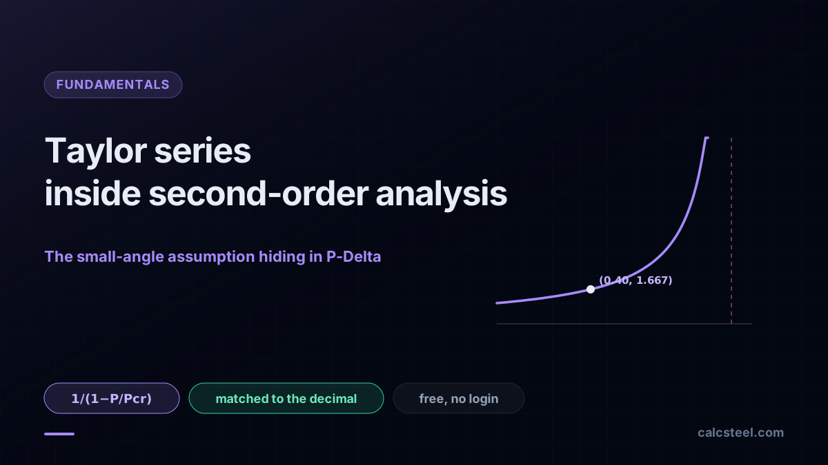
See how the Taylor series hides inside first-order analysis and powers the P-Delta amplifier, matched to a real FEM engine to the decimal. Try it free, no login.
Key takeaways
- First-order analysis is a small-angle truncation: writing equilibrium on the undeformed shape keeps sin theta as theta and cos theta as 1, only the first Taylor term, and the geometry never moves.
- The moment-amplification factor 1/(1 minus P/Pcr) is itself a geometric series 1 + rho + rho squared + rho cubed + ..., one term for every pass of the axial load through the growing deflection.
- On the worked HEB 200 cantilever, first-order gives M0 = 40.0 kNm and delta-1 = 53.29 mm; at rho = 0.400 the amplifier B = 1.667 lifts them to M2 = 66.68 kNm and delta-2 = 88.84 mm.
- The CalcSteel FEM engine matched the hand check to the decimal, and its buckling analysis returned Pcr = 617.32 kN, equal to the Euler closed form pi squared EI/(2L) squared with K = 2 to 0.000%.
- The Taylor remainder is the warning label: near Pcr the amplifier diverges and at large rotations sin theta stops equalling theta, and there the truncation fails and you need full second-order or large-displacement analysis.
The Taylor series has a real job on a leaning steel column
The Taylor series you met in Calculo II usually arrives as a way to approximate a hard function with a polynomial: write sin, or cos, or 1/(1 minus x) as an infinite sum of derivatives, and stop when you are close enough. It looks like a tool for graphs and error bounds, far from a column or a base plate. It is not. Every time an engineer writes equilibrium on the undeformed shape of a structure, they are silently truncating a Taylor series after the first term, and every time they run a second-order analysis, they are keeping the next one.
That is the whole promise of this article. We take one real steel column, lean it under load, and show that the entire ladder from first-order to second-order to full large-displacement analysis is a single Taylor expansion, read at three different truncation depths.
- First-order analysis keeps only the first term: sin theta is theta, cos theta is 1, and the geometry never moves.
- Second-order (P-Delta) analysis keeps the next term: the axial load acting through the sideways deflection, the P times Delta moment.
- The famous amplifier 1/(1 minus P/Pcr) turns out to be a geometric series, one Taylor term per pass of the load through the growing deflection.
Every number here is matched against the CalcSteel FEM engine to the decimal. That is the point of a real engine behind the words: the hand calculation and the machine solution have to meet, and they do. Everything runs free in the browser, so you can rebuild the column yourself while you read.
Three readers will get something different from this. The engineering student gets a concrete reason the Taylor series earns its place in the Calculo I and II ementa. The practising calculista gets a clean mental model of where P-Delta actually comes from. The self-employed calculista gets a free, browser-native way to read a critical load Pcr and form the amplifier without buying a seat of anything.
Taylor and Maclaurin series, the 60-second refresher
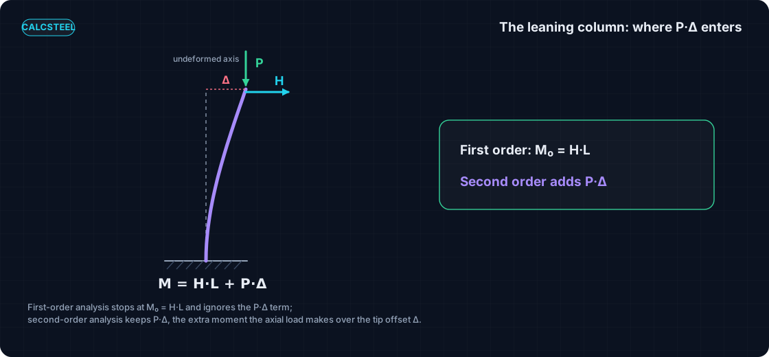
A Taylor series rebuilds a smooth function near a point a from its derivatives at that single point. Write it as f(x) = sum over n of f(n)(a)/n! times (x minus a)n: the value, plus the first derivative times (x minus a), plus the second derivative over 2! times (x minus a)², and so on. When the base point is a = 0 the series gets its own name, the Maclaurin series, and that is the version we will use for sin, cos and 1/(1 minus x).
The picture to keep is this: each added term hugs the true curve over a wider range. Keep one term and you have a horizontal line touching the curve at a; add the next and you have the tangent; add the next and the polynomial starts to bend with the function. Stop early and you have a deliberate approximation, not a mistake.
What tells you how far off you are is the remainder, Rn. The Lagrange form bounds the error of stopping after n terms by the size of the first term you dropped, evaluated somewhere in the interval. That remainder is the honest accounting of a truncation: it says exactly when keeping one term is safe and when it is not. Hold on to it, because the same remainder will later tell a structural engineer when a small-angle assumption stops being harmless.
This is the natural sequel to Calculo I. There you met the ordinary derivative, the single number f'(a). The Taylor series simply stacks all the derivatives at a into one expression that reconstructs the function around that point. Nothing new is being asked of you, only that you keep more of the derivatives you already know how to take.
The small-angle trio: sin theta approximately theta, cos theta approximately 1 minus theta squared over 2, tan theta approximately theta
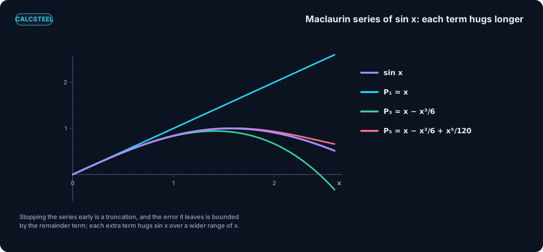
Point the Maclaurin machine at the trigonometric functions and the famous small-angle rules fall straight out. The series are:
- sin θ = θ − θ³/6 + θ&sup5;/120 − ..., so for small θ the first term dominates and sin θ ≈ θ.
- cos θ = 1 − θ²/2 + θ⁴/24 − ..., so cos θ ≈ 1 (or, one term better, 1 − θ²/2).
- tan θ = θ + θ³/3 + 2θ⁵/15 + ..., so tan θ ≈ θ.
These are not rules of thumb pulled from a table. They are Taylor series with every term after the first thrown away, and the angle θ is in radians, which is the only reason the leading coefficient is a clean 1.
How good is the truncation? Here is the error of dropping everything past the first term, as a percentage, at the rotations a real frame actually sees:
| θ | sin θ vs θ error | cos θ vs 1 − θ²/2 error |
|---|---|---|
| 5° | 0.127% | 0.00024% |
| 10° | 0.510% | 0.00392% |
| 20° | 2.060% | 0.06556% |
| 30° | 4.720% | 0.35833% |
Read the first column. At 5° the sin θ ≈ θ approximation is off by about one part in a thousand, and even at 10° it is half a percent. The working frame rotates a few degrees at most under service load, so θ genuinely is sin θ to a fraction of a percent, and the cosine, kept to one more term, is better still. That tiny error is exactly the room in which first-order structural analysis lives.
First-order analysis is a truncated series: equilibrium on the undeformed shape
Now the pivot that the whole article turns on. When you write the equilibrium equations of a structure, sum of moments and sum of forces, on its original, undeformed geometry, you are making two quiet assumptions without naming them. Both are small-angle truncations of a Taylor series.
First, you take cos θ ≈ 1. Physically this says the axial load stays vertical and its lever arm to the joint does not change as the member leans, because the geometry you are writing equilibrium on has not moved. Second, you take sin θ ≈ θ wherever a rotation enters a force balance. Together these keep only the zeroth and first Taylor terms of the trigonometry and discard everything else. The structure in the equations is frozen in its unloaded pose.
That is the precise meaning of first-order analysis: equilibrium on the undeformed shape, which is equilibrium with the small-angle series truncated after the first term. The deflection you compute afterward is a consequence of the loads, but it is never fed back into the geometry that the equilibrium was written on. The load and the shape are decoupled by the truncation.
The important thing is that first-order analysis is not wrong. It is a deliberate truncation whose error you can bound with the same remainder term that bounds any Taylor series, and for the small rotations of a stiff, well-braced frame that error is negligible. The trouble starts only when the discarded terms grow large enough to matter, which is exactly the case second-order analysis is built for. So the honest way to describe first-order analysis is not "the approximate one" but "the one that keeps the first Taylor term."
The linearized elastic line is a binomial-series truncation
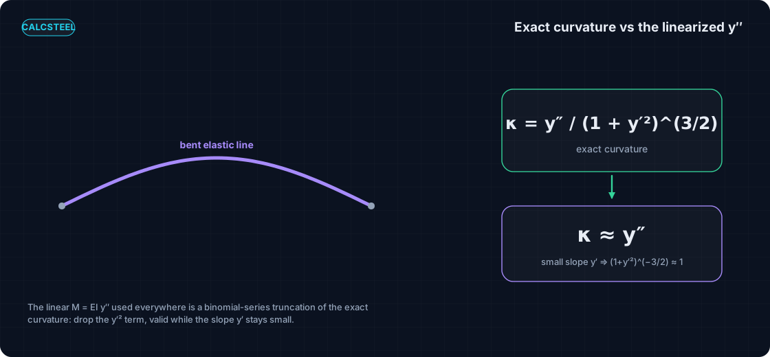
The same truncation is hiding one level deeper, inside the beam equation itself. The exact curvature of a bent member is not the second derivative y″. It is
κ = y″ / (1 + y′²)3/2
where y′ is the slope of the deflected shape. That denominator is what a Taylor series can flatten. Expand (1 + y′²)−3/2 as a binomial series, which is just the Taylor series of (1 + u)−3/2 in u = y′²:
(1 + y′²)−3/2 = 1 − (3/2) y′² + (15/8) y′⁴ − ...
For a member whose slope y′ is small, that is, whose rotation is a small angle, every term past the first is tiny, and the whole factor is ≈ 1. The exact curvature collapses to
κ ≈ y″
which is the linear Euler-Bernoulli relation M = EI y″ that every deflection formula, every stiffness matrix, and every code check quietly assumes. It is the same small-angle truncation as the equilibrium one in the previous section, from the same family of Taylor series, applied to a different quantity. Once you see that M = EI y″ is a truncated series, the rest of the ladder is easy to climb: keep more terms and you get a more honest structure.
Second-order analysis keeps the next term: the P times Delta moment
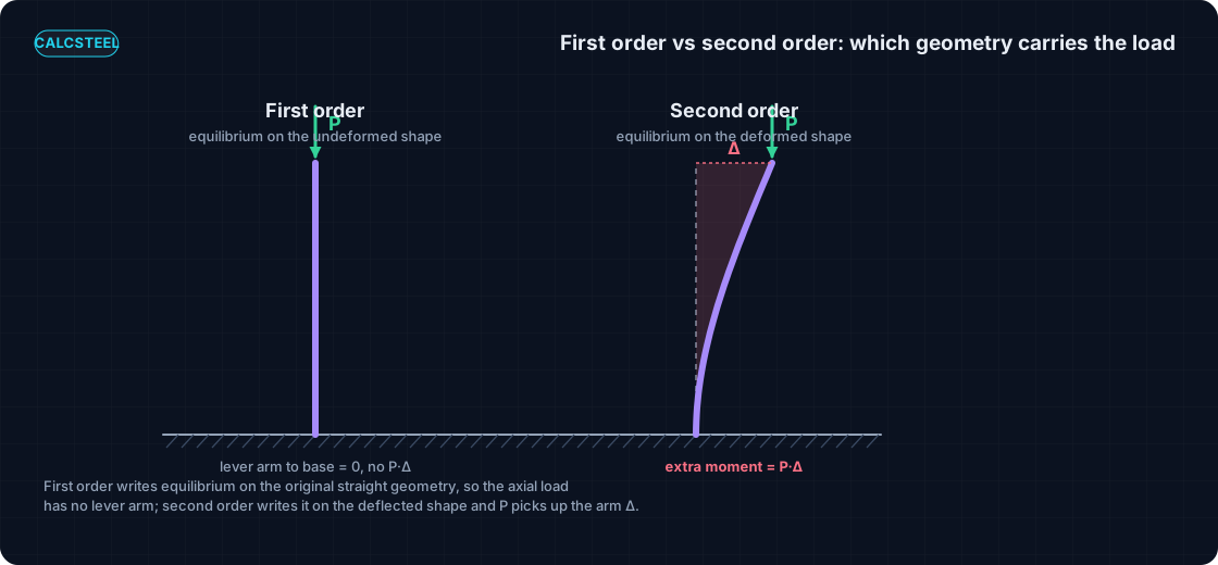
So far every truncation has thrown the higher Taylor terms away. Second-order analysis does the opposite: it keeps the next one. The trick is simply to let the geometry move before writing equilibrium.
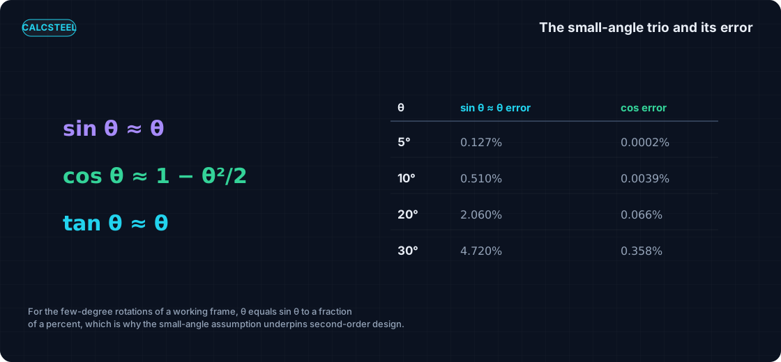
Picture our cantilever column. A lateral load pushes the free top sideways by an amount Δ. In first-order analysis the axial load P slides down a member that, as far as the equations know, is still perfectly vertical, so P contributes no moment at the base. But the real column has leaned. The axial load P now hangs out over the base by the deflection Δ, and it adds a moment
P × Δ
at the fixed base, on top of whatever the lateral load already produced. That extra moment is precisely the term first-order analysis discarded when it froze the geometry. It is the next term in the expansion of equilibrium about the deformed shape: instead of stopping at the undeformed pose, you carry the balance one Taylor step further and let the load act through the displacement it caused.
The name P-Delta comes straight from this product. The load P times the sideways displacement Δ is the second-order moment, and any analysis that includes it is a second-order analysis. Intuitively, the leaning cantilever is the cleanest possible picture: the more it leans, the more the axial load overhangs the base, the more moment it makes, which leans it further. That feedback loop is the whole story, and the next section turns it into a series you already know.
The amplification factor 1/(1 minus P/Pcr) is a geometric series
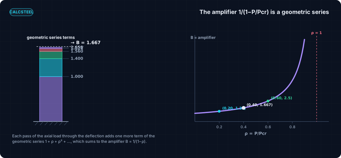
Follow the feedback loop one pass at a time and the amplifier writes itself. Apply the lateral load H and the column deflects to some first-order value Δ0. Now the axial load P, hanging over the base by Δ0, adds a P times Δ0 moment that bends the column further, by an extra Δ1 = Δ0 × ρ, where ρ = P/Pcr is the fraction of the way to the critical load. But that new deflection lets P overhang even more, adding Δ2 = Δ0 × ρ², then Δ3 = Δ0 × ρ³, and so on forever.
The total deflection is the sum of every pass:
Δ = Δ0 (1 + ρ + ρ² + ρ³ + ...)
That parenthesis is a geometric series, the Maclaurin series of 1/(1 minus x) that you met in Calculo II, evaluated at x = ρ. For ρ below 1 it sums to a clean closed form, 1/(1 minus ρ), so
Δ = Δ0 / (1 − ρ)
and the moment amplifies by the very same factor. The amplifier is
B = 1 / (1 − P/Pcr)
and now you can read it for what it is: each pass of the axial load through the growing deflection is one more term of the Taylor series. First-order analysis keeps only the leading 1. Second-order analysis, in its amplified-first-order form, sums the whole series. The Pcr in the denominator is the Euler critical load of the column: the load at which ρ reaches 1, the series stops converging, and the amplifier blows up. That divergence is not a bug in the algebra, it is buckling, told in the language of a Taylor series that has run out of room.
Worked column: first-order vs second-order, checked against the engine
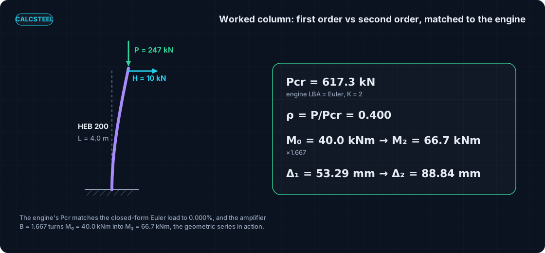
Here is the structure we will carry through the rest of the article, with real numbers and a real engine behind every one of them. It is a steel cantilever column, profile HEB 200, height L = 4.0 m, fixed at the base and free at the top. Bending and buckling both govern about the weak axis, whose second moment of area is Iy = 2001.54 cm⁴, and the steel has E = 20000 kN/cm².
Step 1, the first-order response. Push the free tip sideways with a lateral load H = 10 kN. The base moment is simply H times the height:
M0 = H · L = 10 × 4.0 = 40.0 kNm.
The CalcSteel FEM engine, the same one that runs inside the browser app, returns 40.0000 kNm, a 0.000% difference. The first-order tip deflection of a cantilever is the classic cubic:
Δ1 = H · L³ / (3 E I) = 53.29 mm,
and the engine returns 53.29 mm to every digit, because the cubic beam element is exact for this loading.
Step 2, the Euler critical load. The engine's linear buckling analysis gives Pcr = 617.32 kN. The closed form for a fixed-free column is Pcr = π² E I / (2L)², with effective length factor K = 2 because the free cantilever buckles into a quarter sine wave. That formula gives 617.32 kN. Engine and hand agree to 0.000%.
Step 3, add axial load and amplify. Now press a working axial load P = 247 kN down through the same column. The load ratio is
ρ = P / Pcr = 247 / 617.32 = 0.400,
so the amplifier is B = 1 / (1 − 0.400) = 1.667. Applying it to the first-order results:
M2 = B · M0 = 1.667 × 40.0 = 66.68 kNm, and Δ2 = B · Δ1 = 88.84 mm.
Read that plainly: only 40% of the way to Pcr, second-order effects have added 67% to the first-order moment. The extra 26.68 kNm (that is 66.68 minus 40.0) is nothing other than the sum of every Taylor term past the first. You can watch the geometric partial sums climb toward the amplifier, one term per pass of the load:
| Terms kept | Partial sum of 1 + ρ + ρ² + ... |
|---|---|
| 1 (first-order) | 1.0000 |
| 2 | 1.4001 |
| 3 | 1.5602 |
| 4 | 1.6243 |
| 5 | 1.6499 |
| ∞ | 1.667 |
First-order analysis keeps only the leading 1.0000. Every extra row is one more term of the same series converging on 1.667.
A word of honesty about what the engine did and did not do. The FEM engine gives the exact first-order response and the exact Euler Pcr, matched to the decimal above. The amplifier is the classical closed-form second-order estimate, an amplified first-order elastic analysis (the AISC B1/B2 method), not a separate solve. It is the geometric series in action, and it is accurate precisely while the series converges, which is the subject of a later section.
Try it: buckling and amplification, live
You just watched a geometric series turn into a real moment on paper. Now do it yourself, without picking up a pencil. The calculator embedded right here runs a buckling analysis on a column you define, so the abstract Pcr becomes a number you can push around.
Drop in your own height, profile and end conditions, read the critical load Pcr straight off, then pick a working axial load P and form the ratio ρ = P/Pcr and the amplifier B = 1/(1 − ρ) yourself. Change the height, watch Pcr fall and the amplifier climb. This is the same loop as the worked column: the geometric series 1 + ρ + ρ² + ... made visible.
It is genuinely free, there is no login for the math, and there is no limit on how many times you run it. Explore it the way you would explore a series in Calculo II: change one input, hold the rest fixed, and read how fast the amplifier grows as you approach Pcr.
End conditions (buckling case)
Pinned – Pinned
Cross-section
Slenderness KL/r
134.7
limit 200 · OK
Euler Pcr (elastic)
310.7 kN
Fe = 108.9 MPa
AISC 360 φcPn
245.2 kN
Fcr = 95.5 MPa · elastic
NBR 8800 Nc,Rd
247.7 kN
χ = 0.382 · λ₀ = 1.52
Code vs code — same column
Nc,Rd / φcPn = 1.010
Both codes share the 0.658 / 0.877 buckling curve — the ~1% gap is purely φc = 0.90 (AISC) vs 1/γa1 = 0.909 (NBR).
Demand check — Nd = 150 kN
Step-by-step derivation — live for YOUR column
IPE 200 · L = 3 m · K = 1 · fy = 250 MPa
- 1
Slenderness ratio
λ = K·L/r = 1 × 3000 / 22.28 mm
λ = 134.7 (≤ 200 ✓)
- 2
Euler elastic buckling stress and load
Fe = π²E/λ² = π² × 200,000 / 134.7² · Pcr = Fe·A = Fe × 2854 mm²
Fe = 108.9 MPa · Pcr = 310.7 kN
- 3
Buckling regime (AISC E3)
4.71·√(E/fy) = 4.71·√(200,000/250) = 133.2 < λ = 134.7
elastic buckling → use E3-3 (0.877·Fe)
Elastic range: capacity no longer depends on fy — only geometry (r, K, L) helps.
- 4
AISC 360 critical stress and design capacity
Fcr = 0.877 · Fe = 0.877 × 108.9 = 95.5 MPa · φcPn = 0.9 × Fcr × A
Pn = 272.5 kN · φcPn = 245.2 kN
- 5
NBR 8800 reduction factor and design capacity
λ₀ = √(fy/Fe) = 1.515 > 1.5 → χ = 0.877/λ₀² = 0.382 · Nc,Rd = χ·A·fy/1.1
Nc,Rk = 272.5 kN · Nc,Rd = 247.7 kN
Same 0.658/0.877 curve as AISC — the ~1% difference is φc = 0.90 vs 1/γa1 = 0.909.
Sections that work — 3 lightest of 612 catalog profiles carrying Nd = 150 kN at L = 3 m, K = 1
| Section | kg/m | φcPn (kN) | Nc,Rd (kN) | Util. | |
|---|---|---|---|---|---|
| lightestSHS 80x4 | 9.2 | 164 | 166 | 91% | |
| HSS 76x76x4.8 | 9.9 | 165 | 167 | 91% | |
| CHS 88.9x5 | 10.3 | 172 | 174 | 87% |
Pass criterion: φcPn ≥ Nd (AISC 360 LRFD) AND Nc,Rd ≥ Nd (NBR 8800) AND KL/r ≤ 200, using each section's tabulated-mass area and minimum radius of gyration.
Buckling curve — IPE 200, fy = 250 MPa
Capacity of IPE 200 by unbraced length — K = 1, fy = 250 MPa
| L (m) | KL/r | Pcr Euler (kN) | φcPn AISC (kN) | Nc,Rd NBR (kN) | Regime |
|---|---|---|---|---|---|
| 1 | 45 | 2,796 | 577 | 583 | inelastic |
| 2 | 90 | 699 | 419 | 423 | inelastic |
| 3◀ yours | 135 | 311 | 245 | 248 | elastic |
| 4 | 180 | 175 | 138 | 139 | elastic |
| 5 | 224 ⚠ | 112 | 88 | 89 | elastic |
| 6 | 269 ⚠ | 78 | 61 | 62 | elastic |
| 7 | 314 ⚠ | 57 | 45 | 45 | elastic |
| 8 | 359 ⚠ | 44 | 34 | 35 | elastic |
| 9 | 404 ⚠ | 35 | 27 | 28 | elastic |
| 10 | 449 ⚠ | 28 | 22 | 22 | elastic |
When the small-angle assumption breaks: the remainder term and large displacement
Every truncation has a warning label, and for the Taylor series it is the remainder term. Look back at the small-angle table: the sin θ ≈ θ error was 0.127% at 5° but had grown to 4.720% at 30°. The remainder grows with the angle, and so does the honest question of whether the truncation still holds. There are two distinct ways it can fail.
Failure one, the rotations themselves get large. Slender cables, very flexible members, and form-finding problems can rotate far enough that sin θ is no longer θ: the first dropped Taylor term is now a real fraction of the answer. Here no amplifier saves you, because the linearized geometry that the amplifier is built on has itself expired. You need a true large-displacement, geometrically nonlinear analysis that keeps sin θ whole rather than truncated, and updates the geometry as the structure deforms. This is the regime where the Taylor picture stops being a shortcut and the engine has to carry the full trigonometry.
Failure two, the amplifier's own series stops converging. As the axial load P climbs toward Pcr, the ratio ρ = P/Pcr approaches 1, and the geometric series 1 + ρ + ρ² + ... diverges: B = 1/(1 − ρ) runs off to infinity. Long before it literally diverges, the amplified-first-order shortcut loses accuracy, which is why the codes fence it off. AISC caps the use of the B1/B2 amplifier, and Eurocode EN 1993-1-1 asks for a full second-order analysis whenever the elastic critical ratio αcr = Pcr/P falls below 10. That αcr is just 1/ρ: αcr ≥ 10 means ρ ≤ 0.1, the load is at most a tenth of the way to buckling, the series converges fast, and the small-angle picture is comfortable. When αcr < 10, the load is close enough to Pcr that the higher terms matter and a rigorous second-order solve is required. Our worked column sat at ρ = 0.400, so αcr = 2.5, well inside the region where a rigorous second-order analysis, not a simple amplifier, is the honest choice.
The remainder term is what makes both limits precise rather than a matter of taste. It is the honest warning label printed on the small-angle assumption: safe while the dropped terms are tiny, dangerous the moment they are not.
Where this sits in the calculus-to-structures map
Step back and the whole arc from Calculo I and II lands on real steel, one tool at a time. The ordinary derivative gives the rate of change along a beam, dM/dx equals the shear force V. The second derivative gives the curvature of the elastic line, M = EI y″. The definite integral recovers areas and section properties. The partial derivative gives a deflection straight from the stored energy, as Castigliano's theorem shows. And now the Taylor series gives the second-order amplifier, and reveals that the first-order analysis underneath all the others was a truncation of that same series.
It is one coherent calculus, not a shelf of disconnected tricks. The Taylor series is the tool that finally names the approximation the rest of them were quietly making, and gives you the next term when you need it. If you want to see where the critical load Pcr in the denominator comes from, our Euler buckling post derives it end to end. Same steel, one more member of the calculus family.
From the series to the code check: AISC B1/B2, EC3, NBR 8800
The amplifier is not a classroom curiosity. It is written, almost letter for letter, into the design codes an engineer signs. Every one of them takes the same geometric series and turns it into a required check.
- AISC 360 permits an amplified first-order elastic analysis with two factors: B1 for the member P-δ effect (an axial load acting through the deflection within a member) and B2 for the story P-Δ effect (the load acting through the sway of the whole story). Both are of the form 1/(1 − α Pr/Pe), the same 1/(1 − ρ) series with Pe the elastic buckling load. Chapter C sets out the direct analysis method and Appendix 8 the B1/B2 route.
- Eurocode EN 1993-1-1 keys the whole decision to αcr: if αcr ≥ 10 (elastic) the second-order effects are small enough to ignore or handle by amplification, and below that a fuller second-order analysis is required. That is the convergence test of the series, promoted to a clause.
- ABNT NBR 8800 carries its own B1 and B2 coefficients in the same amplified-first-order spirit, so a Brazilian calculista is summing the identical Taylor series under Brazilian notation.
Two neighbours in the same code family are worth a link. The sway that B2 amplifies has to be triggered in the first place, which is the job of notional loads, small lateral forces that expose an imperfect frame's instability without a full P-Delta run. And the amplified moment does not act alone: it combines with the axial load in the interaction check of combined axial and bending. In every case the point is the same: how many Taylor terms you keep is a code decision, not a vibe. The code tells you when the first term is enough and when you must sum the rest.
Common mistakes and FAQ
The idea is short, which is exactly why the errors are easy to make. Here is the checklist that keeps a second-order estimate honest.
- "Small angle" is not "small deflection." The truncation that first-order analysis makes is on the rotation, not the displacement. A slender cantilever can move its tip a long way (our worked column reached 88.84 mm) while its members still rotate only a few degrees, so sin θ ≈ θ stays valid even though the deflection is visibly large. Confusing the two leads people to distrust a perfectly good analysis, or to trust a bad one.
- Using ρ = P/Pcr with the wrong Pcr. This is the usual real error. The critical load depends on the effective length factor K and on which axis buckles; plug in the strong-axis Pcr, or K = 1 for a column that is really fixed-free (K = 2), and your amplifier is meaningless. Note that our worked column buckled about the weak axis, with Iy = 2001.54 cm⁴, which is the axis that governs. Get Pcr right before you form ρ.
- Second-order is not the same as material nonlinearity. The whole analysis in this article is linear elastic: the steel never yields, Hooke's law holds throughout. Second-order (geometric) nonlinearity is about equilibrium on the deformed shape, a different thing from a nonlinear stress-strain curve. A problem can be one, the other, both, or neither.
- B blows up near Pcr for a real reason. When someone sees 1/(1 − ρ) shoot to infinity they sometimes assume a numerical glitch. It is physics: at ρ = 1 the load has reached Euler buckling, and infinite amplification is the honest mathematical face of an unstable column. Respect the divergence, do not clip it.
- First-order is a truncation, not a mistake. As long as αcr = Pcr/P is comfortable (10 or more in Eurocode terms), keeping only the first Taylor term is a legitimate, code-sanctioned choice. First-order analysis earns its place precisely because the dropped terms are provably tiny there.
Key takeaways
One leaning column, one Taylor series, read at three truncation depths, and every first-order and Euler number matched to a real FEM engine to the decimal.
- First-order analysis is a small-angle truncation. Equilibrium on the undeformed shape keeps sin θ as θ and cos θ as 1, the first Taylor term only, and the geometry never moves.
- The amplifier is a geometric series. B = 1/(1 − P/Pcr) is exactly 1 + ρ + ρ² + ρ³ + ..., one term per pass of the axial load through the growing deflection.
- The worked HEB 200 column. First-order gave M0 = 40.0 kNm and Δ1 = 53.29 mm; at ρ = 0.400 the amplifier B = 1.667 lifted them to M2 = 66.68 kNm and Δ2 = 88.84 mm, 67% more moment only 40% of the way to Pcr.
- The engine matched the hand check to the decimal. Its buckling analysis returned Pcr = 617.32 kN, equal to the Euler closed form π²EI/(2L)² with K = 2 to 0.000%.
- The remainder is the warning label. Near Pcr the series diverges, and at large rotations sin θ stops equalling θ. There the truncation fails and you need full second-order or large-displacement analysis.
Now put your hands on it. Build the column, read Pcr, and form the amplifier yourself in o CalcSteel, a browser-native structural steel design and analysis tool with a genuine FEM engine. The math and the calculators are free, no login, unlimited, and if you are a student the /education offer is free for you. The proof is not a countdown trial; it is a tool you can open right now and check against every number on this page.
Sources
- 1.AISC 360, Specification for Structural Steel Buildings (Chapter C, direct analysis; Appendix 8, B1/B2 amplified first-order)
- 2.Eurocode EN 1993-1-1, Design of steel structures: General rules (5.2 second-order effects and the elastic critical ratio alpha-cr)
- 3.ABNT NBR 8800, Projeto de estruturas de aco (B1/B2 coefficients, second-order analysis)
- 4.Timoshenko and Gere, Theory of Elastic Stability (Euler load, beam-column amplification)
- 5.Stewart, Calculus (Taylor and Maclaurin series, the remainder term)
Try CalcSteel for free
Model, analyze and design steel structures in your browser. No install, no signup.
Open the 3D editor