Stress in a String: Why a Tension-Only Member Has Just One Number, with a Worked Check
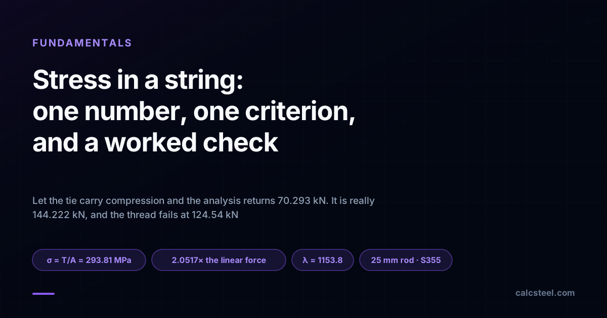
A string is the one member in structural engineering where “the stress” really is a single number. It has no bending stiffness and no compression capacity, so the stress tensor collapses to σ = T/A and every yield criterion returns the same answer. That is the gift. The trap is that a member which cannot push is a nonlinear member, and a linear analysis that lets the tie push returns 70.293 kN where the real force is 144.222 kN. This article works one braced bay end to end on the CalcSteel engine, and ends with a rod whose thread fails at 124.54 kN.
Key takeaways
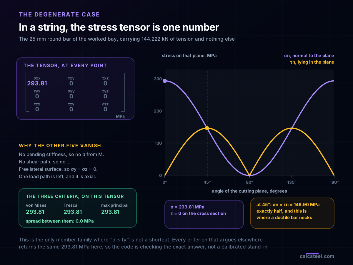
- In a string the stress tensor has exactly one non-zero component. σ = T/A, and σy, σz, τxy, τyz and τzx are all identically zero. On the worked rod σ = 293.81 MPa, and von Mises, Tresca and maximum principal stress all return 293.81 MPa, with a spread of 0.0 MPa between them.
- That is why “σ ≤ fy” is not a shortcut here. Everywhere else in a steel member the code checks a calibrated stand-in for a six-component object. In a tie it is checking the exact criterion, because the criteria have nothing left to disagree about.
- One number does not mean one plane. Cut the same rod at 45 degrees and you read σn = τn = 146.90 MPa, exactly half of σ. That is where a ductile bar necks, and it is the reason the shear limit of steel is fy/√3 rather than fy.
- A string cannot push, and that makes it nonlinear. Left in a linear model, the compressed diagonal of the worked bay carries 73.930 kN of compression it cannot carry: its Euler load is 0.728 kN, so the model overstates its capacity by a factor of 101.6.
- Remove it and the tension in the surviving rod goes from 70.293 kN to 144.222 kN, a factor of 2.0517. The storey drift goes from 6.628 mm to 13.599 mm, the same factor to four decimals, and crosses the H/400 limit of 10.0 mm on the way.
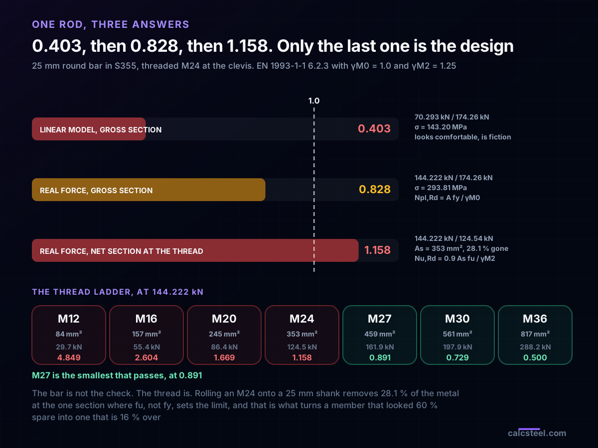
- The bar is not the check. The thread is. An M24 thread on a 25 mm shank removes 28.1 % of the metal at the one section where fu, not fy, sets the limit. Npl,Rd = 174.26 kN on the gross section, Nu,Rd = 124.54 kN on the thread, and the demand is 144.222 kN. The member fails at 1.158.
- AISC's flat 0.75 factor for threaded rods is the thread area ratio in disguise. Across M12 to M36 the ratio As/Ab runs from 0.745 to 0.803, so 0.75 is that geometry rounded down, and it stops being an arbitrary coefficient the moment you compute it.
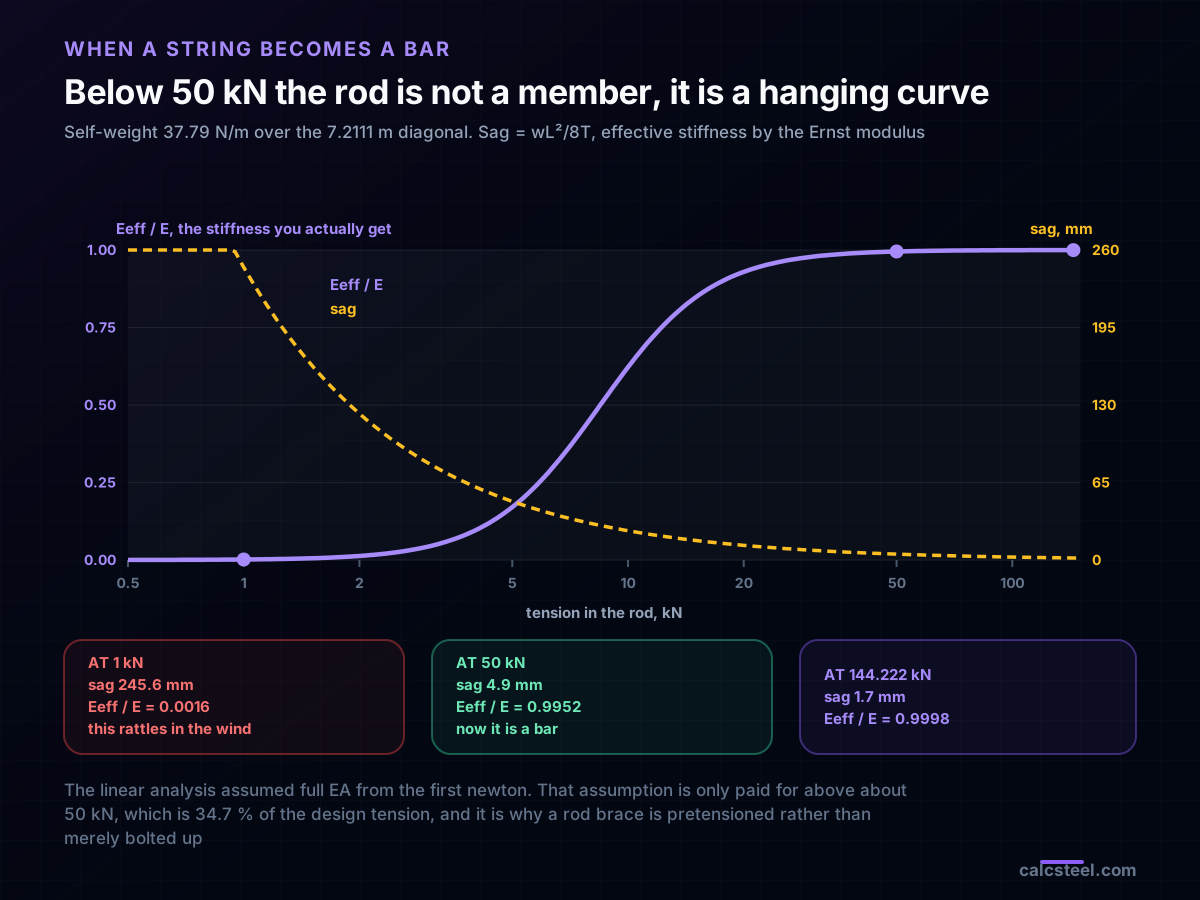
- A slack string is not a member at all. At 1 kN of tension the 7.2111 m rod sags 245.6 mm and delivers 0.16 % of its axial stiffness. It reaches 99 % of EA only above about 50 kN, which is 34.7 % of the design tension, and that is the engineering case for pretensioning a rod brace instead of merely bolting it up.
A brace that passes at 0.40 and fails at 1.16
Here is a bay you could model in five minutes. Six metres wide, four metres tall, HEA 200 columns, an IPE 300 beam, simple connections everywhere, and a pair of crossed 25 mm round bars taking 120 kN of storey shear. It is the most ordinary piece of steelwork in the world.
Draw the two rods, run the analysis, read the answers. The tension diagonal carries 70.293 kN. Against a 25 mm bar in S355, whose plastic tension resistance is 174.26 kN, that is a utilisation of 0.403. The storey drift is 6.628 mm against an H/400 limit of 10.0 mm. Everything passes with room to spare.
Every one of those numbers is wrong, and they are wrong because of a single modelling decision nobody consciously made. The other diagonal came back at -73.930 kN. It is in compression. A 25 mm rod spanning the 7.2111 m diagonal has an Euler load of 0.728 kN. The model asked it to carry a hundred times what it can, and it quietly did, because a linear stiffness matrix has no way of knowing that a rod is a string.
Take that rod out, which is what physically happens, and the surviving diagonal carries 144.222 kN. Utilisation on the gross section 0.828. Drift 13.599 mm, over the limit. And then check the thread, because the rod is threaded M24 at the clevis, and the resistance there is 124.54 kN. Utilisation 1.158. The brace fails.
Three answers came out of one member: 0.403, 0.828, 1.158. This article is about why the first one appeared, why the stress in a string is the simplest stress state in all of mechanics and yet produces the most expensive modelling mistake in a steel frame, and what the code is actually checking when it checks one number.
What a string is, mechanically
In physics a string is an idealisation with two properties, and it is worth stating them as prohibitions rather than as features, because the prohibitions are what the analysis has to respect.
It has no bending stiffness. EI is taken as zero, so it cannot carry a moment, cannot resist curvature, and takes whatever shape the loads give it. A thread hanging from a hook is straight; hang a weight halfway along and it becomes two straight segments; distribute the weight and it becomes a catenary. The geometry is an output, not an input.
It cannot push. Tension only. Try to shorten the distance between its ends and it does not resist, it goes slack. There is no negative branch of its force-displacement curve, only a flat one at zero.
A real steel tie rod is not a string. It has a genuine EI, it will carry a small moment, and if you compress it hard enough it will resist right up to its buckling load. The question is not whether the idealisation is exact but whether the errors it makes are small. For the rod in the worked bay the slenderness L/r is 1153.8. Codes cap compression members at 200 and tension members at 300. At 1153.8 the flexural stiffness is not small, it is irrelevant: the rod is a string to within the precision of anything you could measure.
That is the test to apply. A member is a string when its slenderness is high enough that EI stops mattering, and in steelwork that covers rod bracing, cable bracing, sag rods, hangers, tie-downs and most of what holds a canopy on.
The stress tensor of a string, and why it is one number
Stress at a point in a solid is a second-order tensor: nine components, six of them independent once moment equilibrium forces symmetry. Asking for “the stress” without naming a plane is normally an incomplete question, because the answer changes with the orientation of the cut.
In a string it is not incomplete, and it is worth seeing exactly why each component dies.
- σx = T/A. The one survivor. The axial force divided by the area, uniform across the section because there is no moment to make it vary.
- No σ from bending. EI is zero, so M is zero, so the My/I term that fills a beam's section with a linear stress gradient is simply absent.
- τxy = τxz = 0. Shear in a member comes from the gradient of the moment. No moment, no gradient, no VQ/It.
- σy = σz = τyz = 0. The lateral surface of the rod is free. Nothing is pressing on it, so the transverse normal stresses vanish at the surface and, in a slender member with no transverse load, everywhere else too.
What is left is a tensor with a single non-zero entry. On the worked rod, with T = 144.222 kN and A = 490.87 mm², that entry is σ = 293.81 MPa and the other eight are zero to machine precision.
The consequence is the point of this whole article. A yield criterion is a rule for turning six numbers into one, and the reason there is more than one criterion is that reasonable rules disagree. On this tensor they cannot. The principal stresses are (293.81, 0, 0). Von Mises returns 293.81 MPa. Tresca returns 293.81 MPa. Maximum principal stress returns 293.81 MPa. The sim computes all three and asserts the spread between them is below 10⁻⁹ MPa; it comes out at exactly 0.0.
So when the code writes σ ≤ fy for a tie, it is not applying a calibrated stand-in for something more complicated, the way it is when it checks a beam's extreme fibre and quietly ignores the shear acting there. For a string, σ ≤ fy is the criterion. This is the only member family where that is literally true.
One number does not mean one plane
There is a trap inside the good news. A single-component tensor is not a state in which nothing happens on other planes. It is a state in which the components on other planes are all determined by one number, which is a different claim.
Sweep the cutting plane through the rod. On the cross section, normal to the axis, you read σn = 293.81 MPa and τn = 0: pure tension, no shear, which is why the cross section is the plane everyone draws. Rotate the cut by 45 degrees and the same state reads σn = 146.90 MPa and τn = 146.90 MPa. Rotate to 90 degrees, cutting along the axis, and both are zero.
The 45 degree plane carries the maximum shear anywhere in the material, and its value is exactly σ/2. That is not a coincidence of this rod, it is the geometry of a uniaxial state: with principal stresses (σ, 0, 0), the radius of Mohr's circle is σ/2 and the circle passes through the origin.
Two things follow that are worth carrying around. First, a ductile steel coupon pulled to failure necks and shears on planes close to 45 degrees, and the cup-and-cone fracture surface you get out of a tensile test machine is a picture of this sweep, not of the axial stress. Second, the shear strength of steel comes out of the same algebra. Set von Mises equal to fy in pure shear and you get τ = fy/√3 = 0.577 fy, which is the number behind AISC's 0.6 Fy and behind the Vpl,Rd of EN 1993-1-1. The string is where that relationship is easiest to see, because in a string the maximum shear is visibly half the thing you already computed.
The worked bay, and what the engine was asked
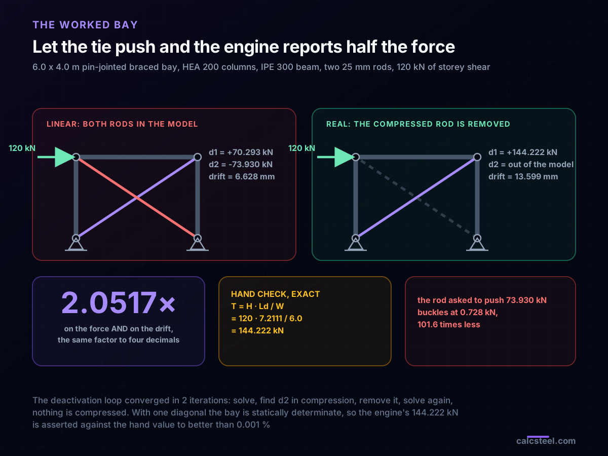
The model is deliberately plain. Four nodes, both bases pinned, a 6.0 m by 4.0 m bay, HEA 200 columns, an IPE 300 beam with pinned ends, and two crossed 25 mm round bars with pinned ends, so the bay is a genuine truss and every member carries axial force only. A single horizontal load of 120 kN is applied at the top left node.
Before trusting anything the engine says about this bay, the same script runs a calibration: a simply supported IPE 400 under a uniform load, checked against wL²/8, wL/2 and 5wL⁴/384EI. All three match to six decimal places. That is the gate; nothing below is quoted unless it passes.
The bay is then solved twice. Once with both diagonals in the model, which is what a linear analysis does by default. Once with the deactivation loop that the CalcSteel API actually runs on tie members: solve, look for any tie in compression, remove it from the model, solve again, and stop when nothing is compressed. On this bay the loop converged in two iterations. The first solve found d2 at -73.930 kN, removed it, and the second solve found nothing left in compression.
Note what deactivation means: the member is removed, not softened. There is no reduced modulus, no small residual stiffness, no compression-only spring. A slack rod contributes nothing at all, and the honest way to model nothing is to take it out.
With one diagonal the bay becomes statically determinate, which is what makes this example worth publishing: the answer is checkable by hand, exactly. Sum moments and you get T = H · Ld / W = 120 · 7.2111 / 6.0 = 144.222 kN, with the beam at -120 kN and the leeward column at -80.0 kN. The engine returns all three, and the sim asserts each against the closed form to better than 0.001 %.
What the linear model got wrong, in detail
The linear run is not obviously broken. It satisfies equilibrium: the two diagonals together deliver (70.293 + 73.930) · 6.0/7.2111 = 120.0 kN of horizontal shear, which is exactly the applied load. It satisfies compatibility. Nothing in the output is flagged. Read it and you would sign the bay off.
What it violates is a constitutive fact: one of those members cannot carry the force assigned to it. The 25 mm rod on the 7.2111 m diagonal has I = 19 174.8 mm⁴ and r = 6.25 mm, so its Euler load is π²EI/L² = 0.728 kN. The model gave it 73.930 kN of compression. That is 101.6 times its buckling capacity, and 0.5 % of the tension the other rod actually has to carry.
Once the fiction is removed the numbers move together:
- Tension goes from 70.293 kN to 144.222 kN, a factor of 2.0517.
- Drift goes from 6.628 mm to 13.599 mm, a factor of 2.0517 to four decimals, because removing one of two identical springs halves the lateral stiffness of the bay.
- The serviceability check flips. H/400 on a 4.0 m storey is 10.0 mm. The linear model passes at 6.628 mm. The real bay does not, at 13.599 mm.
Reverse the load and the picture is symmetric: d1 goes slack, d2 picks up 144.222 kN, and the sim asserts the magnitude is identical. This is the reason both rods are there. They are not sharing the load, they are taking turns, and each one has to be sized for the whole of it. A cross brace is two members doing one member's job in two directions, and a linear analysis reads it as two members sharing one job, which is the same drawing and the opposite engineering.
σ = T/A, and the section where it is not A
With the force settled, the stress is arithmetic. A 25 mm round bar has A = πd²/4 = 490.87 mm², and the sim asserts the registry's area against that closed form rather than trusting the table. So:
σ = T/A = 144 222 N / 490.87 mm² = 293.81 MPa
Against fy = 355 MPa that is a utilisation of 0.828, and by the argument in the previous sections that single number is the complete stress state of the member. Compare it with what the linear model would have given: 143.20 MPa, utilisation 0.403. Same rod, same code clause, same steel.
But 490.87 mm² is not the area everywhere. A tie rod has to attach to something, and the usual detail is a thread at each end into a clevis or a turnbuckle. Thread an M24 onto a 25 mm shank and the section that resists is not the shank, it is the thread's tensile stress area: As = 353 mm² from ISO 898-1. That is 28.1 % of the metal gone, at the one section where the load is highest and the geometry is a stress raiser.
Which is why the codes check tension members twice, and why the two checks use different materials properties and different safety factors. It is not belt-and-braces, it is two genuinely different failure modes.
What the code actually checks, in both families
EN 1993-1-1 §6.2.3 asks for the smaller of two resistances.
Gross section yielding. Npl,Rd = A fy / γM0 = 490.87 · 355 / 1.0 = 174.26 kN. This is a ductility limit state: the whole member goes plastic, stretches visibly, and redistributes. It is checked against fy with γM0 = 1.0.
Net section rupture. Nu,Rd = 0.9 Anet fu / γM2 = 0.9 · 353 · 490 / 1.25 = 124.54 kN. This is a fracture limit state at one section, with no warning and no redistribution, which is why it uses fu, the harsher γM2 = 1.25, and the additional 0.9. The 0.9 is not a rounding: it is the calibration that keeps the rupture check less likely than the yielding check, so that a member which is overloaded yields first and tells you.
For the worked rod the resistance is min(174.26, 124.54) = 124.54 kN against a demand of 144.222 kN. Utilisation 1.158. It fails.
AISC 360 arrives in the same place by a different route. Chapter D2 gives φPn = 0.90 Fy Ag for yielding and 0.75 Fu Ae for rupture, which for a Grade 50 rod with Fu = 450 MPa gives 152.42 kN and 119.14 kN, governing at 119.14 kN and a utilisation of 1.211. For threaded rods specifically, table J3.2 lets you skip the net area and use Fnt = 0.75 Fu on the gross bolt area instead, which here gives 124.25 kN, within 0.3 % of the European net-section answer.
That flat 0.75 is worth a second look, because it usually reads as an arbitrary coefficient. It is not. Compute As/Ab across the whole metric coarse series and you get 0.745 at M12, 0.780 through the middle of the range, and 0.803 at M36. AISC's 0.75 is that geometric ratio rounded down to its conservative end. The specification is telling you the same thing ISO 898-1 is, in one number instead of a table.
The fix on this bay is arithmetic once you know which check governs. The required stress area is 144 222 · 1.25 / (0.9 · 490) = 408.8 mm², so M27 with As = 459 mm² is the smallest thread that works, at a utilisation of 0.891. The shank grows to 30 mm to carry it. The bar got 44 % heavier because of a few centimetres at each end.
Why the rod cannot push, quantified
Everything above depends on one claim: that the compressed diagonal contributes nothing. It is worth putting a number on it rather than asserting it, because “the tie goes slack” is the kind of statement that gets believed without being checked.
The rod is 25 mm in diameter over a 7.2111 m diagonal, pinned at both ends. Its radius of gyration is d/4 = 6.25 mm, so the slenderness is 1153.8. For comparison, EN 1993-1-1 and most national annexes recommend keeping compression members below 200 and tension members below 300; this is nearly four times the looser of the two limits. In non-dimensional terms λ̄ = 15.47, where column curves stop being drawn.
The Euler load follows: Ncr = π²EI/L² = π² · 200 000 · 19 174.8 / 7 211.1² = 0.728 kN. Set that beside the tension resistance of the same rod, 174.26 kN, and the ratio is 239.4. Set it beside the force the member actually has to carry, 144.222 kN, and the compression capacity is 0.5 % of it.
In other words the rod is not merely weaker in compression, it is absent. Zero is a better model of 0.728 kN, in a bay where the working force is 144 kN, than 0.728 kN is. Modelling it as a tension-only member is not a conservative simplification; it is the accurate one.
You can see the collapse for yourself. Put the same 25 mm circular section into the buckling calculator below with a 7.2111 m length and pinned ends, and watch the capacity fall off the bottom of the chart. Then shorten it to 1 m and watch it come back. Nothing about the material changed; only L² did.
End conditions (buckling case)
Pinned – Pinned
Cross-section
Slenderness KL/r
134.7
limit 200 · OK
Euler Pcr (elastic)
310.7 kN
Fe = 108.9 MPa
AISC 360 φcPn
245.2 kN
Fcr = 95.5 MPa · elastic
NBR 8800 Nc,Rd
247.7 kN
χ = 0.382 · λ₀ = 1.52
Code vs code — same column
Nc,Rd / φcPn = 1.010
Both codes share the 0.658 / 0.877 buckling curve — the ~1% gap is purely φc = 0.90 (AISC) vs 1/γa1 = 0.909 (NBR).
Demand check — Nd = 150 kN
Step-by-step derivation — live for YOUR column
IPE 200 · L = 3 m · K = 1 · fy = 250 MPa
- 1
Slenderness ratio
λ = K·L/r = 1 × 3000 / 22.28 mm
λ = 134.7 (≤ 200 ✓)
- 2
Euler elastic buckling stress and load
Fe = π²E/λ² = π² × 200,000 / 134.7² · Pcr = Fe·A = Fe × 2854 mm²
Fe = 108.9 MPa · Pcr = 310.7 kN
- 3
Buckling regime (AISC E3)
4.71·√(E/fy) = 4.71·√(200,000/250) = 133.2 < λ = 134.7
elastic buckling → use E3-3 (0.877·Fe)
Elastic range: capacity no longer depends on fy — only geometry (r, K, L) helps.
- 4
AISC 360 critical stress and design capacity
Fcr = 0.877 · Fe = 0.877 × 108.9 = 95.5 MPa · φcPn = 0.9 × Fcr × A
Pn = 272.5 kN · φcPn = 245.2 kN
- 5
NBR 8800 reduction factor and design capacity
λ₀ = √(fy/Fe) = 1.515 > 1.5 → χ = 0.877/λ₀² = 0.382 · Nc,Rd = χ·A·fy/1.1
Nc,Rk = 272.5 kN · Nc,Rd = 247.7 kN
Same 0.658/0.877 curve as AISC — the ~1% difference is φc = 0.90 vs 1/γa1 = 0.909.
Sections that work — 3 lightest of 612 catalog profiles carrying Nd = 150 kN at L = 3 m, K = 1
| Section | kg/m | φcPn (kN) | Nc,Rd (kN) | Util. | |
|---|---|---|---|---|---|
| lightestSHS 80x4 | 9.2 | 164 | 166 | 91% | |
| HSS 76x76x4.8 | 9.9 | 165 | 167 | 91% | |
| CHS 88.9x5 | 10.3 | 172 | 174 | 87% |
Pass criterion: φcPn ≥ Nd (AISC 360 LRFD) AND Nc,Rd ≥ Nd (NBR 8800) AND KL/r ≤ 200, using each section's tabulated-mass area and minimum radius of gyration.
Buckling curve — IPE 200, fy = 250 MPa
Capacity of IPE 200 by unbraced length — K = 1, fy = 250 MPa
| L (m) | KL/r | Pcr Euler (kN) | φcPn AISC (kN) | Nc,Rd NBR (kN) | Regime |
|---|---|---|---|---|---|
| 1 | 45 | 2,796 | 577 | 583 | inelastic |
| 2 | 90 | 699 | 419 | 423 | inelastic |
| 3◀ yours | 135 | 311 | 245 | 248 | elastic |
| 4 | 180 | 175 | 138 | 139 | elastic |
| 5 | 224 ⚠ | 112 | 88 | 89 | elastic |
| 6 | 269 ⚠ | 78 | 61 | 62 | elastic |
| 7 | 314 ⚠ | 57 | 45 | 45 | elastic |
| 8 | 359 ⚠ | 44 | 34 | 35 | elastic |
| 9 | 404 ⚠ | 35 | 27 | 28 | elastic |
| 10 | 449 ⚠ | 28 | 22 | 22 | elastic |
When a string is not yet a bar
There is one more assumption hiding in the analysis, and it is the reverse of the first. The linear model wrongly let the rod push. It also assumed the rod delivers its full axial stiffness EA from the first newton of tension, and that is not true either.
A rod hung across a diagonal carries its own weight. The 25 mm bar masses 3.85 kg/m, so w = 37.79 N/m over 7.2111 m. Under a tension T it hangs in a catenary with a sag of approximately wL²/8T. Pull an extra millimetre out of the ends and part of that goes into straightening the curve rather than stretching the steel, so the stiffness you actually get is lower than EA. The standard way to write that down is the Ernst effective modulus, Eeff = E / (1 + w²L²AE/12T³), and its behaviour is dramatic because T appears cubed.
- At 1 kN the rod sags 245.6 mm and delivers Eeff/E = 0.0016. It is a hanging curve with a bolt on each end, and in wind it will slap.
- At 10 kN the sag is 24.6 mm and Eeff/E = 0.6221. Better, and still 38 % short of the stiffness the model assumed.
- At 50 kN the sag is 4.9 mm and Eeff/E = 0.9952. This is the first row in the sweep above 0.99, and it is 34.7 % of the design tension.
- At the design tension of 144.222 kN the sag is 1.7 mm and Eeff/E = 0.9998. Here the string genuinely is a bar.
So the linear elastic assumption is earned, not free. It is earned above roughly a third of the design load, which is exactly the engineering case for pretensioning a rod brace with a turnbuckle rather than merely bolting it up and trusting the wind to take up the slack. The pretension is not there to make the rod stronger. It is there to make the model true.
Where the one-number picture stops being true
The clean answer holds for the free length of a straight, taut, axially loaded tie. It is worth naming the places it does not, because those are where ties actually fail.
At the ends. A clevis, a fork or a welded lug clamps the rod and forces it to bend when the geometry moves. Bending returns, so σ from M returns, and it is superimposed on the full σ = T/A of the free length. It is a local effect over a length of a few diameters, and it is one reason ties get detailed with pins rather than fixed bolts.
At the thread. The section change is a stress raiser, and the local peak is well above the 408.6 MPa you get by dividing the force by As. For static design the code handles it by using fu and γM2, as above. For a brace that sees thousands of load reversals, fatigue at the first engaged thread is a separate check with its own detail category, and it is where rod braces actually break.
Under transverse load. The moment a rod carries anything across its length, including its own weight at low tension, the shape becomes part of the problem. That is the catenary regime of the previous section, and it is a geometrically nonlinear problem, not a stress problem.
In the surrounding structure. Removing a member changes the load path everywhere, not only in the brace. In the worked bay the beam went from -58.487 kN to -120.0 kN and the leeward column from -38.991 kN to -80.0 kN when d2 came out. If you correct the brace and leave the beam and columns on the old numbers, you have moved the error rather than fixed it.
How to model a tie so this does not happen
Six things, in the order they matter.
- Declare the member a tie, not a bar. In CalcSteel that is the class kind; in any other package it is the tension-only or no-compression flag. If the software has no such flag, model one diagonal per load direction and run both.
- Check the sign of every diagonal in the output. A tie reporting compression is not a small error to be noted; it is the analysis telling you it solved a different structure.
- Do it per load case, not once globally. A rod that is slack under wind from the left is working under wind from the right. Deactivating it for the whole model would be as wrong as leaving it in.
- Size both rods for the full force. They take turns; they do not share.
- Check the thread, not the bar. Nu,Rd on the tensile stress area is the governing resistance for almost every threaded tie, and it is the one people skip.
- Recheck drift after the correction. Halving the bracing stiffness moves serviceability, and drift is often what governs a braced bay in the end.
And one thing not to do: do not model the tie as a very soft bar to “help it converge”. A small residual compression stiffness puts a force into a member that is physically slack, which shows up as an equal and opposite error somewhere else in the frame. Remove it or keep it; there is nothing sensible in between.
The simplest stress state, and the costliest modelling error
There is a nice symmetry to how this one goes wrong. The string is the easiest object in mechanics of materials. Its stress tensor has one entry, every yield criterion agrees on it, and the check the code writes is the criterion itself rather than a calibrated approximation of it. If stress analysis were the hard part, ties would be the safest members in a building.
The difficulty is not in the stress, it is in the force. Getting T requires the analysis to know something a stiffness matrix has no way to express: that this member has no negative branch. Leave that out and every number downstream is wrong by a factor of two, and each of them is individually plausible.
The bay in this article passed three checks it should have failed. It read 0.403 on the brace when the answer was 0.828 on the gross section and 1.158 at the thread. It read 6.628 mm of drift against a 10.0 mm limit when the real figure was 13.599 mm. And it did all of that while satisfying equilibrium exactly, which is why nothing in the output looked wrong.
So the practical version of everything above fits in one line. In a string the stress is one number, and the whole job is making sure it is the right one.
Sources
- 1.EN 1993-1-1 §6.2.3, tension members: Npl,Rd = A fy / γM0 and Nu,Rd = 0.9 Anet fu / γM2, and the slenderness recommendations for ties
- 2.EN 1993-1-8, design of joints: threaded rods, clevis and pin connections, and the partial factor γM2 = 1.25 for rupture
- 3.AISC 360, Specification for Structural Steel Buildings, chapter D2 (tensile yielding and tensile rupture) and table J3.2 (Fnt = 0.75 Fu for threaded rods)
- 4.ISO 898-1 and ISO 261, coarse metric threads: the tensile stress area As from M12 to M36, the external anchor for every net-section number here
- 5.ABNT NBR 8800, Projeto de estruturas de aço e de estruturas mistas de aço e concreto, tension member and slenderness provisions
- 6.Gere and Goodno, Mechanics of Materials (uniaxial stress, Mohr's circle for a state with one non-zero principal stress, and the 45 degree plane)
- 7.Irvine, Cable Structures (the catenary, sag under self-weight, and the transition from a slack cable to an axially stiff member)
- 8.Ernst, Der E-Modul von Seilen unter Berücksichtigung des Durchhanges (the effective modulus of a sagging tie used in the stiffness sweep)
Try CalcSteel for free
Model, analyze and design steel structures in your browser. No install, no signup.
Open the 3D editor