The Derivative as a Rate of Change: Why dM/dx Equals the Shear Force in Every Beam
The single most useful fact in beam analysis, dM/dx = V, is a derivative. This guide connects the derivative as a rate of change from Calculus I and II to the shear and bending moment diagrams every structural engineer draws, with three engine-verified examples and a live calculator.
Key takeaways
- The shear force is the derivative of the bending moment: dM/dx = V. It is the Calculus I derivative-as-a-rate-of-change, read as the slope of the moment diagram, not a separate structural rule.
- Its partner is dV/dx = minus w, and together they give d2M/dx2 = minus w: the load is the second derivative of the moment, which is why moment diagrams under uniform load are concave-down parabolas.
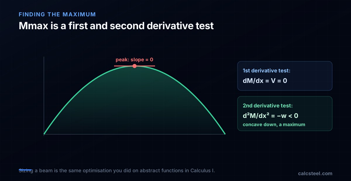
- Finding the maximum moment is an optimisation problem: it sits where the shear (first derivative) crosses zero, confirmed by the negative second derivative, exactly the first and second derivative tests.
- The rule has an asterisk: the maximum can also sit at a fixed support (an endpoint) or a point load (a non-differentiable corner), where the shear is not zero, the endpoint and corner cases calculus tells you to check.
- Read backwards it is Calculus II: the moment is the integral of the shear, and the change in moment equals the area under the shear diagram, which is the fundamental theorem of calculus on a beam.
- We proved it on the real FEM engine: the finite-difference derivative of the solver's moment diagram lands on its own shear to 0.0 error over 24 stations, because a computer does the same calculus, numerically.
Every beam diagram you draw is a calculus problem
Somewhere in the first year of an engineering degree, two courses run in parallel and never quite shake hands. In one room you learn the derivative as a rate of change: the slope of a curve, the limit of a difference quotient, the thing that tells you how fast one quantity moves when another one does. In another room you learn to draw shear force and bending moment diagrams for beams, following a recipe of cuts and equilibrium. Most students finish both without ever being told that they are the same subject.
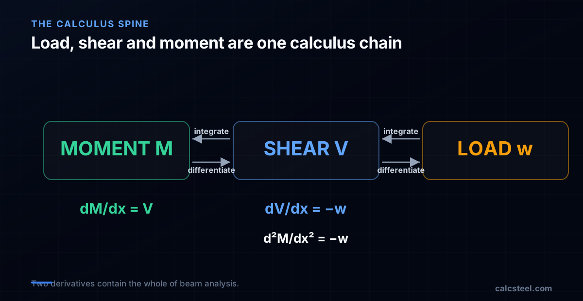
They are. The single most useful fact in beam analysis, dM/dx = V, is a derivative. It says the shear force at any point is the rate of change of the bending moment along the beam, the slope of the moment diagram read off with the exact tool you met in Calculus I. Its partner, dV/dx = −w, says the load is the rate of change of the shear. Stack them and you get d²M/dx² = −w: the bending moment is a function whose second derivative is the load, which is why moment diagrams curve the way they do.
This guide is the bridge between the two rooms. It is written for the student who can differentiate x² but has never seen why that skill draws a parabola on a beam, and for the practising or self-employed engineer who wants the clean mental model behind the diagrams they produce every day. Every worked number below was computed by the CalcSteel finite element engine and checked against the calculus by hand, and there is a live calculator further down so you can watch the derivative move. If diagrams themselves are new to you, the companion guide on shear force and bending moment diagrams covers the drawing; this one is about the calculus underneath.
The derivative, in the one sentence structures needs
Strip away the notation and a derivative answers one question: if I nudge the input a little, how fast does the output respond? That ratio, output change over input change, is a rate of change. Geometrically it is the slope of the tangent line to a curve. Formally it is that slope in the limit as the nudge shrinks to zero:
f′(x) = limΔx→0 [ f(x + Δx) − f(x) ] / Δx
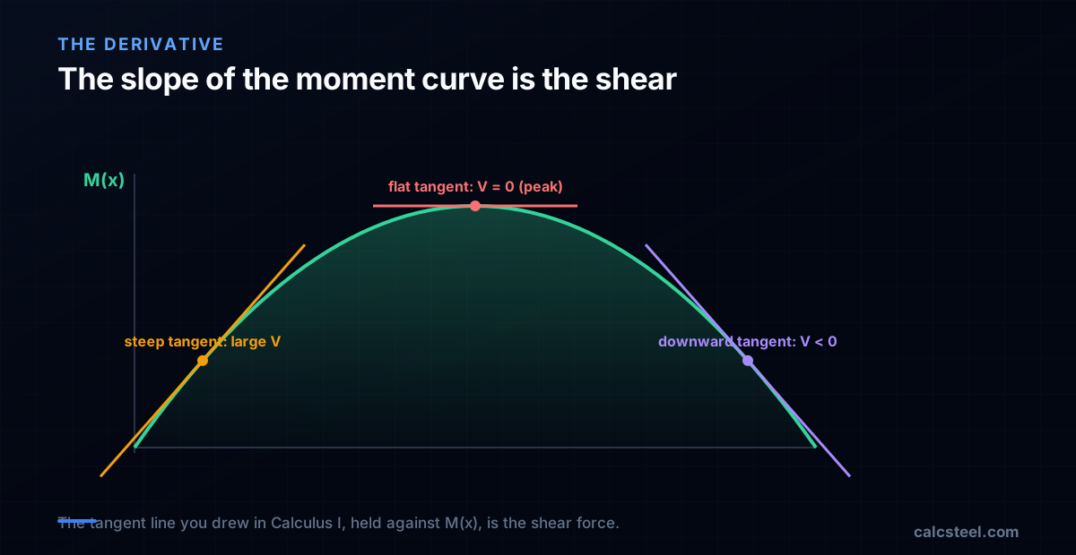
Three readings of the same idea, and each one has a job in this article. The rate of change reading is the physics: how fast the moment builds as you walk along the beam. The slope of the tangent reading is what you literally see: hold a ruler against the moment diagram and its steepness is the shear. The limit of a difference quotient reading is how a computer does it: sample the curve at two nearby points, divide the rise by the run, and shrink the run. We will use that last one to prove dM/dx = V numerically on a real solver.
Two consequences of the definition carry the whole method. First, where a smooth curve reaches a peak or a valley its tangent is flat, so its derivative is zero: this is how you find a maximum. Second, the derivative can itself be differentiated. The second derivative measures how the slope is changing, which is curvature, or concavity: positive second derivative curves a graph upward like a bowl, negative curves it downward like a dome. Hold on to both. The zero-derivative peak is how we locate the maximum moment, and the sign of the second derivative is why a moment diagram under uniform load is a dome and not a bowl.
The two relations that turn load into moment
Take a short slice of a loaded beam, of length dx, and write equilibrium for that slice: sum of vertical forces zero, sum of moments zero. Shrink the slice toward zero length and the two equilibrium statements become two derivatives. This is the one place in a structures course where the limit definition from calculus is doing visible work, and the result is the entire toolkit:
- dV/dx = −w. The slope of the shear diagram at any point is the negative of the distributed load there. No load means a flat shear line; a uniform load w means the shear falls at a constant rate w per metre.
- dM/dx = V. The slope of the moment diagram is the shear at that point. This is the sentence to keep: the shear is the derivative of the moment. Where the shear is large the moment climbs steeply; where the shear is zero the moment is momentarily flat.
Substitute the first into the second and the moment obeys a single second-order relation:
d²M/dx² = dV/dx = −w
That is the compact reason a moment diagram has the shape it has. Under a downward uniform load w is positive, so d²M/dx² is negative, so the moment diagram is concave down, a dome, for the whole loaded length. Under no distributed load the second derivative is zero, so the moment diagram is straight: that is why the moment under a lone point load is made of straight lines, not curves. The order of the curve is set by calculus alone: constant load gives a parabolic moment, a linearly varying load gives a cubic, and no load gives a line. You are reading the antiderivative of the load, twice over.
Worked example 1: the derivative, proved on a real beam
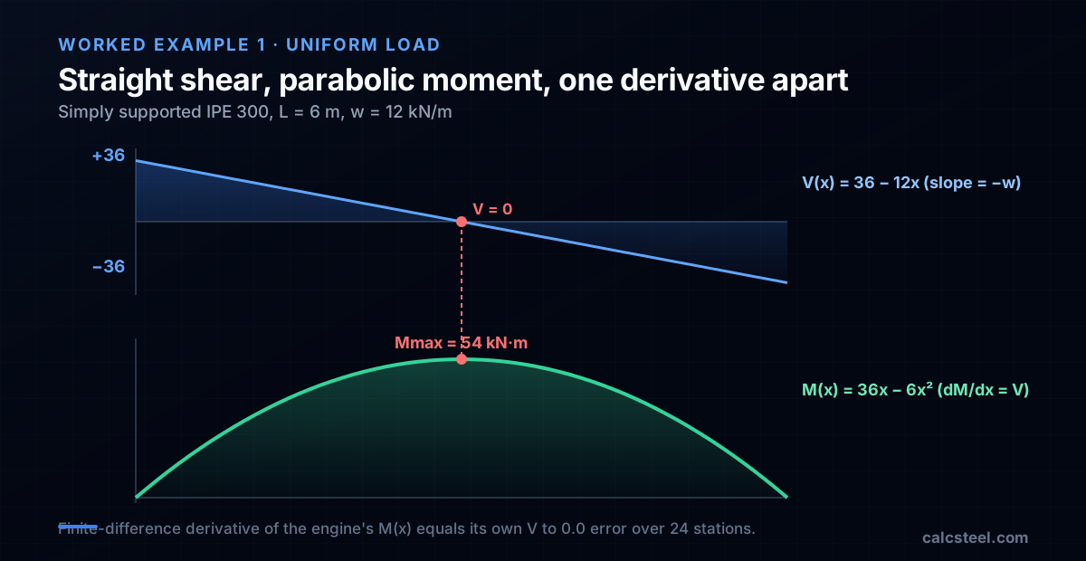
Here is the clean case that shows every idea at once. Take a simply supported IPE 300 spanning L = 6 m, carrying a uniform load w = 12 kN/m. Pin at one end, roller at the other. By symmetry each reaction is half the total load: R = wL/2 = 12 × 6 / 2 = 36 kN, which the CalcSteel engine returns to the digit at both supports.
The shear is a straight line, because its derivative is constant
Walk from the left support. The shear starts at +36 kN and, because dV/dx = −w = −12, falls by 12 kN for every metre travelled: V(x) = 36 − 12x. It is a straight line of slope −12, exactly the load. It crosses zero at x = 3 m, the midspan.
The moment is a parabola, and its slope is the shear
Because dM/dx = V, the moment is the running integral of that shear line: M(x) = 36x − 6x². That is a downward parabola, and its peak is where its derivative, the shear, is zero, at x = 3 m. The value there is M = 36(3) − 6(9) = 54 kN·m, the textbook wL²/8 = 12 × 36 / 8 = 54. The engine agrees to the digit.
The proof: the solver's own diagram differentiates to its own shear
This is where calculus stops being a story. We ran the beam through the FEM engine, sampled its moment diagram at 24 stations along the span, and took the finite-difference slope between neighbouring stations, the difference quotient [M(x+Δx) − M(x)] / Δx with Δx = 0.25 m. At every single interval that numerical derivative of the moment landed exactly on the shear the engine reported at the same place. Near the left support the moment climbs at 34.5 kN·m per metre and the shear there is 34.5 kN. Just before midspan the moment climbs at 1.5 and the shear is 1.5. The worst disagreement across all 24 intervals was 0.0. The derivative of the moment diagram is not like the shear force; it is the shear force, and a numerical solver reproduces the identity without ever being told it.
Finding the maximum: the first and second derivative tests
The whole reason an engineer draws these diagrams is to find one number, the maximum bending moment, because it sizes the beam. Calculus hands you the procedure directly, and it is the same optimisation you did with abstract functions in Calculus I.
First derivative test: the peak is where the shear is zero
A smooth function reaches a local maximum where its derivative changes from positive to negative. The derivative of the moment is the shear, so the moment peaks where the shear crosses zero. In the uniform-load beam above, the shear V(x) = 36 − 12x runs positive, hits zero at x = 3 m, then goes negative: a maximum, and M = 54 kN·m sits exactly there. Finding Mmax is solving V(x) = 0. That is all the famous rule is.
Second derivative test: which way does it curve
To confirm a zero-slope point is a peak and not a trough, calculus checks the second derivative: negative means concave down, a maximum. For the beam, d²M/dx² = −w = −12, which is negative, so the stationary point is a maximum. It also fixes the shape: the moment diagram domes downward under the load, and its curvature is literally the load intensity. A heavier load is a sharper dome.
The point of inflection is the point of contraflexure
Where a curve switches concavity, its second derivative passes through zero: a point of inflection. On a beam that is the point of contraflexure, where the bending moment changes sign and the beam stops sagging and starts hogging, flipping which face is in tension. The same Calculus I idea, an inflection where f″ = 0, tells a designer which flange to brace along each stretch of a continuous beam.
One honest caveat the calculus insists on: the first-derivative test only finds peaks on the smooth parts of the curve. The true maximum can also sit at an endpoint or at a point where the function is not differentiable. That exception is not a footnote here, it is the next worked example.
Worked example 2: the corner where the derivative breaks
Replace the spread load with a single one. The same 6 m simply supported beam now carries a point load P = 24 kN at midspan. Each reaction is P/2 = 12 kN, from the engine.
Straight lines, because the load is zero between the ends
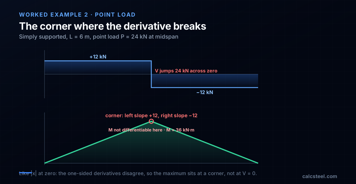
Away from the load there is no distributed load, so dV/dx = −w = 0 and the shear is constant: +12 kN across the left half, −12 kN across the right. And because d²M/dx² = −w = 0 on each half, the moment has zero curvature: it is made of straight lines. The moment ramps up at a slope of +12 to a peak of M = PL/4 = 24 × 6 / 4 = 36 kN·m under the load, then ramps back down at −12. Two straight lines meeting at a point, and the engine matches the 36 kN·m to the digit.
At the load, the moment is not differentiable
Now the calculus subtlety. The moment diagram has a sharp corner under the point load. Approach x = 3 m from the left and the slope is +12; approach from the right and it is −12. The two one-sided derivatives disagree, so the derivative does not exist at that point: the moment is not differentiable at the load, in exactly the way |x| is not differentiable at zero. The shear diagram shows the same fact as a vertical jump of 24 kN, from +12 to −12, a step discontinuity precisely the size of the load.
Our numerical check caught this cleanly. The finite-difference derivative of the moment matched the shear to 0.0 everywhere except the one interval straddling the load, where it spiked by exactly 12 kN·m per metre, the signature of a corner the difference quotient cannot smooth over. This is why the “maximum is where the shear is zero” rule needs its asterisk: here the shear never passes through zero at all, it jumps across it, and the maximum sits at the non-differentiable corner. You find it by inspection, not by setting a derivative to zero.
Running it backwards: the moment is the integral of the shear
Calculus II is the same relation read in the other direction. If the shear is the derivative of the moment, then the moment is the integral of the shear, and the fundamental theorem of calculus makes that quantitative:
M(b) − M(a) = ∫ab V dx
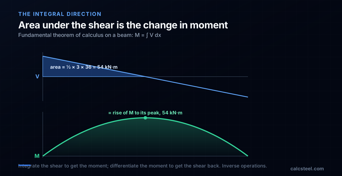
In plain terms: the change in bending moment between two points equals the area under the shear diagram between them. This is the fastest hand check in structural analysis, and it is nothing but the fundamental theorem applied to a beam.
Test it on the uniform-load beam. Between the support and midspan the shear diagram is a triangle: base 3 m, height 36 kN, area = ½ × 3 × 36 = 54 kN·m. That area is the rise in moment from 0 at the support to 54 at midspan, matching the peak exactly. On the point-load beam the shear is a rectangle over the left half: 12 kN × 3 m = 36 kN·m, again the peak. The two directions are consistent because they are inverse operations: differentiate the moment and you get the shear; integrate the shear and you get the moment back.
This is also why the moment diagram is one polynomial degree higher than the shear, and the shear one degree higher than the load. Integration raises the degree: a constant load integrates to a linear shear and a quadratic moment. When you sketch a bending moment diagram by eye, you are integrating the shear diagram in your head, accumulating its area as you move along the beam.
See the derivative move: the live calculator
The fastest way to feel dM/dx = V is to change the beam and watch both diagrams respond together. The calculator below is the real CalcSteel shear and moment tool, embedded right here. Drag the load, switch between a point load and a uniform load, move the supports, and the shear and moment diagrams redraw instantly.
Two things to try. Set a uniform load and watch the moment diagram peak sit locked to the point where the shear line crosses zero: that is dM/dx = V finding the maximum in real time. Then switch to a point load and watch the smooth peak snap into a sharp corner while the shear jumps: that is the derivative breaking at the load, the second worked example made live. Recreate example 1 (6 m span, 12 kN/m) and confirm the 54 kN·m peak for yourself.
It is the real tool, not a teaser: unlimited runs, free, and no login needed for the math. If it opens in its own tab, here is the direct link to the shear and moment diagram calculator. For a full member with reactions, deflection and section sizing together, the free beam calculator is the next step.
|V| max
30 kN
@ x = 6 m
M max (sagging)
45 kN·m
@ x = 3 m
M min (hogging)
-0 kN·m
@ x = 6 m
Reactions (kN)
R_A 30 · R_B 30
Simply supported beam — uniformly distributed load
Segment equations — x in m, from the left end
0 m ≤ x ≤ 6 m
V(x) = 30 − 10·x [kN]
M(x) = 30·x − 5·x² [kN·m]
Profiles that resist this moment
Md = 45 kN·m → required Wx = Md / (fy/γa1) = 45 kN·m / (250/1.1) = 198 cm³
Bending screen (Wx ≥ Md/(fy/γa1), NBR 8800 γa1 = 1.10 — AISC 360 φb = 0.90 is nearly identical); plastic Zx is valid for compact sections only. δ is the elastic deflection of THIS loading with E = 200 GPa and the section's Ix (loads taken at service value). LTB, shear, compactness and code deflection limits are verified on the profile page and in the 3D editor. "Open in 3D editor" recreates THIS beam — span, supports and every load — with the profile already assigned.
Worked example 3: sign, the fixed end, and the asterisk on the rule
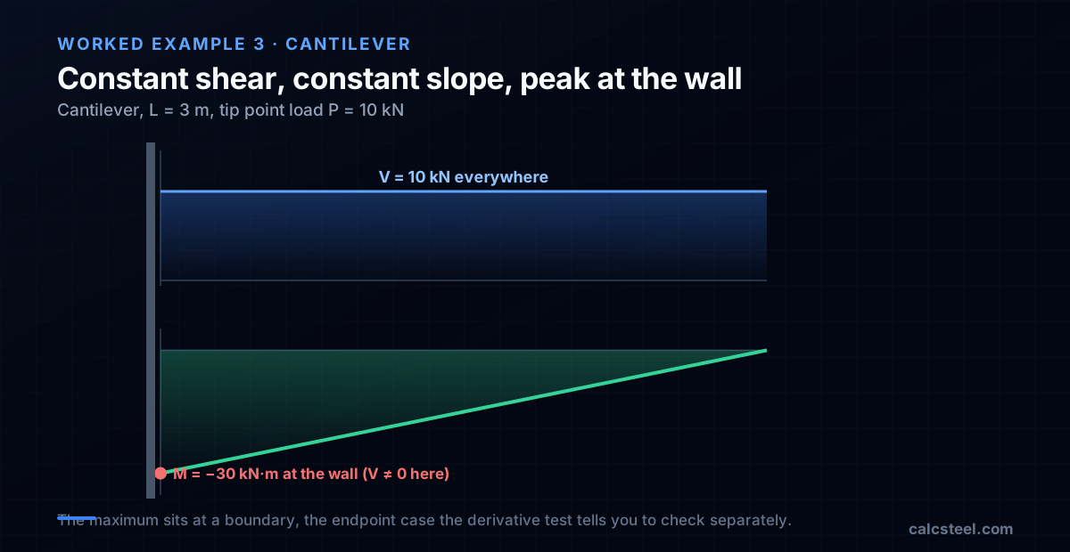
One more case to settle the sign and the exception. A cantilever, built in at the wall, spans L = 3 m and carries a tip point load P = 10 kN. There is one support, the fixed end, and the engine reports its reactions: a 10 kN vertical force and a 30 kN·m moment.
Constant shear, constant slope
The shear is the same everywhere along the cantilever: the full 10 kN is carried from the tip back to the wall, with no distributed load to change it (dV/dx = −w = 0). Because dM/dx = V = 10, a constant, the moment diagram is a straight line of constant slope 10. It runs from 0 at the free tip to −30 kN·m at the wall, and the finite-difference derivative of the engine's moment diagram sits on 10 kN at every station, worst error 0.0. Constant derivative, straight line: the calculus is unmistakable.
The maximum is at the wall, where the shear is not zero
Here the shear never reaches zero, yet the moment clearly has a maximum: 30 kN·m in magnitude, right at the fixed end. This is the asterisk on the first-derivative test. The rule “the peak is where V = 0” only governs the smooth interior of a span. The true maximum can also live at a boundary, and a fixed support is exactly that, a boundary of the domain, precisely the endpoint case Calculus I warns you to check separately when you optimise. On a cantilever the governing moment is always at the wall, and reading only “V = 0” would point you at the wrong section entirely.
The negative sign is the sagging-versus-hogging distinction: a negative moment here means hogging, the top fibre in tension, the opposite of the sagging midspan of the simply supported beams. The sign of M is not decoration, it tells you which flange is in tension and therefore which one to check for bracing.
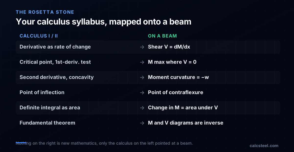
Your Calculus I and II syllabus, mapped onto a beam
Almost every headline topic from a first-year calculus sequence has a direct structural meaning. If you are studying both at once, this is the Rosetta stone. Nothing on the structures side is new mathematics, it is the calculus you already have, pointed at a beam.
- Limits and the difference quotient (Calc I): the cut-a-slice-of-length-dx-and-shrink-it argument that turns beam equilibrium into dV/dx and dM/dx. The whole method starts with a limit.
- The derivative as a rate of change (Calc I): the shear force is the rate of change of the moment along the beam. dM/dx = V, literally.
- Critical points and the first-derivative test (Calc I): the maximum moment is where the shear (the first derivative) crosses zero. Sizing a beam is an optimisation problem.
- The second derivative, concavity and inflection (Calc I): d²M/dx² = −w sets the curvature of the moment diagram, and its inflection point is the point of contraflexure where sagging becomes hogging.
- Endpoint and non-differentiable extrema (Calc I): the moment can peak at a fixed support (a boundary) or at a point load (a corner), the exact cases the optimisation checklist tells you not to forget.
- The definite integral as area (Calc II): the change in moment is the area under the shear diagram.
- The fundamental theorem of calculus (Calc II): differentiating the moment and integrating the shear are inverse operations, which is why the two diagrams are locked together.
- Antiderivatives and polynomial degree (Calc II): integrating a constant load up to a linear shear and a quadratic moment is why load, shear and moment climb one polynomial degree at a time.
The payoff is that you do not have to memorise beam diagrams as a separate recipe. If you understand the derivative as a rate of change and the integral as accumulated area, the diagrams are a direct consequence, and a tool like CalcSteel is just doing the calculus faster than you can.
Four things students get wrong about dM/dx = V
1. Thinking the maximum moment is always where the shear is zero
True only on the smooth interior of a span. The maximum can sit at a fixed support (an endpoint) or at a point load (a non-differentiable corner), where the shear is not zero at all. Always check the boundaries and the load points, exactly as you would when optimising any function.
2. Confusing the derivative with the function
A large shear does not mean a large moment. The shear is the slope of the moment, not its value. At the support of a simply supported beam the shear is at its maximum while the moment is zero, because a steep slope starting from zero has not accumulated any height yet. Slope and value are different things.
3. Forgetting the units of a rate of change
A derivative has the units of output over input. dM/dx is a moment (kN·m) divided by a length (m), which is kN, a force: the shear. If a “dM/dx = V” check ever comes out in the wrong units, the equation is being misapplied. The dimensions confirm the calculus.
4. Believing a computer does something other than calculus
A finite element solver does not escape the derivative, it approximates it numerically, exactly the difference quotient from the limit definition evaluated on a fine mesh. That is why the engine's moment diagram differentiates back to its own shear to zero error: the software is doing your Calculus I homework, just at a few thousand stations per second.
How CalcSteel turns the calculus into a diagram
Under the hood, the CalcSteel engine is applied calculus. It never draws a curve it has not computed: it solves the beam or frame for the internal forces, then reports the shear and moment as functions of position, the same V(x) and M(x) you would integrate by hand, evaluated at every node of the model.
- It solves, then samples. The finite element method breaks the member into elements and solves equilibrium and compatibility. The shear and moment come out at every station, which is why differentiating the moment diagram numerically hands you the shear back, as the worked examples showed to zero error.
- The peak is found, not guessed. Because Mmax is where the shear crosses zero (or a boundary, or a load), the engine locates it the way calculus prescribes, and the calculator highlights it as you drag the load.
- The same math scales to a frame. On a single beam you can integrate by hand. On a continuous beam or a portal frame the equations become indeterminate and hand integration runs out, but the underlying relation dM/dx = V still holds at every point, and the solver keeps applying it. See the beam-to-frame walkthrough for where hand methods stop and the engine takes over.
The practical takeaway for a student or a working engineer is the same: the diagrams are not a separate skill to memorise. They are the derivative and the integral you already know, drawn on a beam. Open the calculator, change a load, and watch the calculus happen.
Sources
- 1.Hibbeler, R.C., Structural Analysis (relations between load, shear and moment)
- 2.MIT OpenCourseWare 18.01 Single Variable Calculus (derivatives, the FTC, optimisation)
- 3.Gere & Goodno, Mechanics of Materials (shear-force and bending-moment relationships)
- 4.AISC Steel Construction Manual, 16th Edition (beam design from the governing moment)
Try CalcSteel for free
Model, analyze and design steel structures in your browser. No install, no signup.
Open the 3D editor