Stress–Strain Curve of Steel: Elastic to Fracture
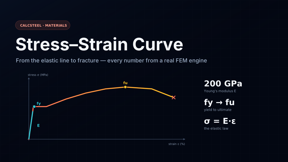
The steel stress–strain curve, explained from elastic line to fracture: yield strength, Young's modulus, ductility and design. Try the free calculator.
Key takeaways
- The curve is the material's fingerprint: one tension test fixes E, fy, fu and ductility across five regions — elastic, yield, strain hardening, necking, fracture.
- The elastic line is Hooke's law (σ = Eε): the FEM engine recovered E = 200.00 GPa (A36) and 210.00 GPa (S355) at every load level, to five significant figures.
- Same stiffness, different strength: every structural steel shares E ≈ 200–210 GPa, so a higher grade buys a higher yield point, not less deflection — and usually costs ductility (fu/fy falls from 1.60 to 1.17).
- The plastic plateau is design capacity: for an IPE 330, My = Sx·fy = 171.5 kN·m and Mp = Wpl·fy ≈ 201.6 kN·m — an 18% shape-factor bonus, if the section is compact.
- Real members sit on the curve: a portal-frame rafter at σ = 209.8 MPa, utilisation 0.84, lives on the elastic straight-line below the knee — exactly what the editor's green colours show.
The one graph that defines a steel
Grip a machined steel specimen at both ends, mount it in a universal testing machine, and pull — slowly, relentlessly — until it snaps. The machine records two things the whole way: how hard it is pulling (force) and how much the bar is stretching (elongation). Normalise those by the bar's cross-section and its original length and you get a single graph, the stress–strain curve. That one curve is the fingerprint of the material. Read off its shape and you have — all at once — the stiffness E, the yield strength fy, the ultimate strength fu, and the ductility that tells you whether the steel will warn you before it breaks.
This is the definitive walk along that whole curve, from the straight elastic line where steel behaves like a perfect spring, through yield, strain hardening and necking, all the way to fracture. Every number you will see here was computed by the CalcSteel FEM engine and then hand-checked — the elastic modulus recovered to five significant figures, the yield and plastic moments of a real IPE 330, and a real portal-frame rafter placed exactly where it sits on the curve. There is a live, unlimited Mohr's circle calculator embedded further down so you can drive the maths yourself.
We wrote this for three readers at once:
- The student who needs the definitions to actually stick — proportional limit, 0.2% proof stress, shape factor — with worked numbers behind each one.
- The practising engineer who already knows the theory but wants it tied cleanly to design: elastic vs plastic section modulus, section classification, and utilisation on a real member.
- The curious — anyone who has seen the classic curve in a textbook and wants to understand, physically, what each bend in it means.
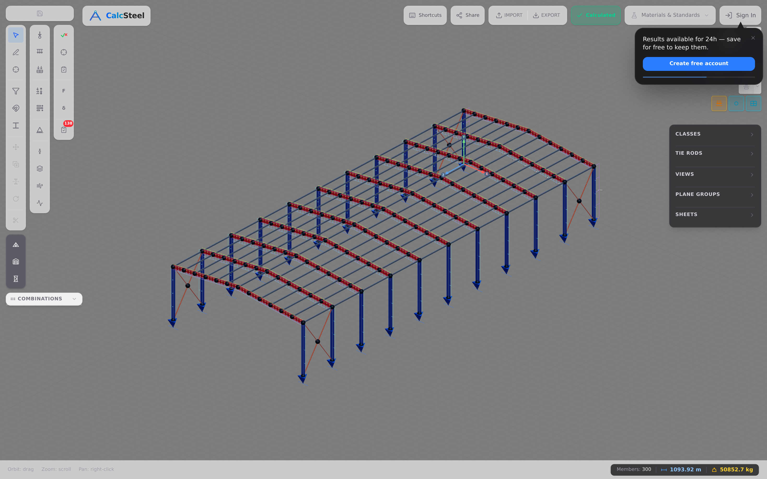
CalcSteel is a free, browser-native structural steel design and analysis solution running a genuine FEM engine — the same engine that produced the numbers below. Nothing to install; the frame in the figure above is exactly the kind of model where this curve stops being an abstraction and starts carrying load.
What the stress–strain curve actually is
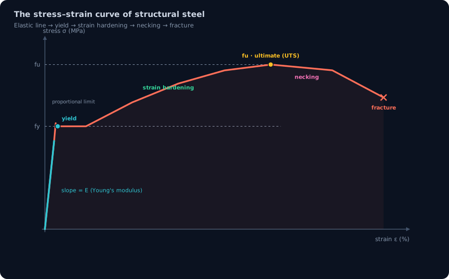
A stress–strain curve plots stress against strain from a tension test. Stress σ is force divided by the specimen's cross-sectional area; strain ε is elongation divided by its original length. As you pull harder, the curve traces how the steel responds — and its shape reveals the material's stiffness, strength and ductility in a single picture.
Look at the axes. The vertical axis is stress, in MPa (megapascals — force per unit area; a modulus like E is large enough that we quote it in GPa). The horizontal axis is strain, which is dimensionless — a length divided by a length — so we read it as a percentage. A strain of 0.1% simply means the bar got 0.1% longer. Because stress carries the units and strain does not, the slope of the curve — stress over strain — comes out in MPa or GPa, and that slope is Young's modulus.
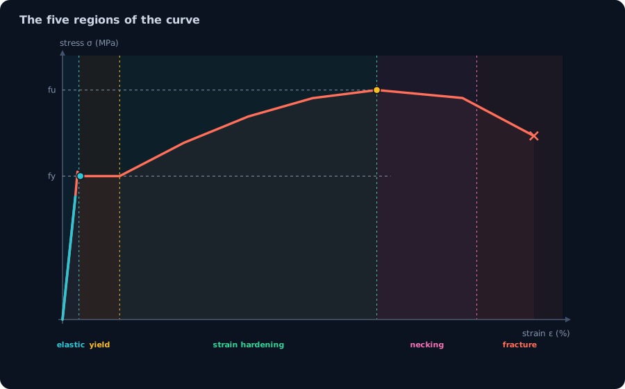
Every structural steel traces the same five regions along that curve, in order:
- Elastic — a straight line; the steel behaves like a spring and springs fully back.
- Yield — the material begins to flow; for mild steel this shows up as a distinct, flat plateau.
- Strain hardening — the steel fights back and stress climbs again to a peak.
- Necking — a local waist forms and the engineering stress falls.
- Fracture — the specimen breaks, and how far it stretched first is its ductility.
The rest of this article walks each region in turn, and — crucially — connects it to what you do at the desk: sizing a beam, checking a utilisation, choosing a grade. The curve is not a lab curiosity; it is the boundary condition on every member you design.
Where the curve came from
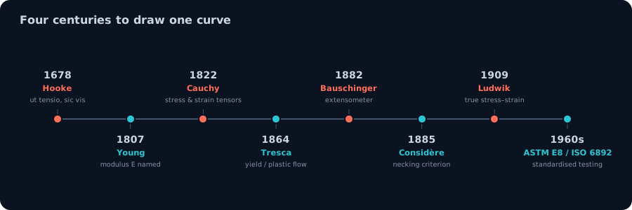
The stress–strain curve looks obvious once you know it, but it took roughly three and a half centuries and a chain of remarkable people to assemble. The pieces arrived in a logical order: first the linear law, then the material constant that scales it, then the language of stress and strain, and finally the parts of the curve beyond the straight line.
- 1678 — Robert Hooke. The foundation: ut tensio, sic vis — "as the extension, so the force." Deformation is proportional to load. That is the straight elastic line, three hundred years before we drew it that way.
- Early 18th century — Leonhard Euler. Works with an elastic-modulus concept in ratio form, sharpening the idea that stiffness is a fixed proportion between force and deflection.
- 1807 — Thomas Young. The proportionality constant is named — Young's modulus, E — the slope of the elastic line and the single most important number the curve gives us.
- 1822 — Augustin-Louis Cauchy. Formalises the tensors of stress and strain, giving the axes of our graph their rigorous, general definitions.
For context, the earliest structural thinking predates all of this — Galileo (1638) and later Mariotte (1660s) wrestled with how beams break long before anyone could describe stress properly. But the modern curve needed its non-linear regions explained, and that came later still:
- 1864–1870 — Henri Tresca. Studies plastic flow and yielding, giving us the first workable yield criterion — the physics of what happens when the straight line ends.
- 1882 — Johann Bauschinger. Builds a precision extensometer that could actually resolve small strains, and discovers the Bauschinger effect — that yielding in one direction lowers the yield stress in the reverse direction.
- 1885 — Armand Considère. States the instability criterion for necking — why and when the specimen forms its waist near the peak.
- 1909 — Paul Ludwik. Introduces true stress–strain, correcting for the shrinking cross-section and explaining why the true curve keeps rising while the engineering curve falls.
- 20th century — standardisation. The test itself is pinned down by ASTM E8 and ISO 6892, so a curve measured in one lab means the same thing in another.
Every region we are about to walk was somebody's life's work. The payoff is that today a single tensile test — governed by those standards — hands you E, fy, fu and ductility together.
The five regions of the curve
Walk the curve from left to right and it passes through five distinct regions, each governed by different physics. Here is each one, in order, with the technical landmark it defines.
1. Elastic region
The opening straight line. Stress and strain rise in exact proportion, and the slope of that line is Young's modulus E. This is Hooke's law in action: σ = Eε. Anything you deform here is fully recoverable — unload the bar and it springs back to its original length with no permanent set. The region ends at two closely-spaced landmarks: the proportional limit, where the line stops being perfectly straight, and just above it the elastic limit, the last stress from which the steel still returns completely to zero strain. For design, this is the region you want your structure to live in.
2. Yield
The material stops behaving elastically and starts to flow. Mild hot-rolled steel does this dramatically: it shows a sharp upper yield point, then drops to a lower yield point and runs along a nearly flat yield plateau while Lüders bands sweep across the specimen. Because the plateau is so flat and clear, mild steel gives you an unambiguous yield strength fy — you read it straight off. (Steels without this sharp knee need the 0.2% offset method, which we cover later.)
3. Strain hardening
Past the plateau the steel toughens up: its internal structure rearranges and it resists more load again, so the curve climbs a second time to its highest point. That peak is the ultimate tensile strength fu (UTS) — the maximum engineering stress the material sustains. The height of this climb above yield is the material's reserve strength beyond first yield.
4. Necking
At the peak an instability sets in: deformation localises and a visible waist, or neck, forms. Because the cross-section is now shrinking fast, the engineering stress — always computed on the original area — begins to fall, even though the material at the neck is still hardening. Corrected for the real, reduced area, the true stress keeps rising right up to the break. This engineering-versus-true distinction trips people up constantly, so keep it in mind.
5. Fracture
The neck thins until the specimen breaks. The total elongation at fracture — how far the bar stretched before it let go — is a direct measure of ductility. A steel that stretches a long way before fracture warns you; a brittle one snaps with little notice.
Five landmarks to carry forward: the proportional limit (end of linearity), the elastic limit (end of full recovery), the yield strength (onset of permanent flow), the UTS (peak engineering stress), and fracture (the end, and the measure of ductility). Everything that follows — the worked elastic line, the offset yield, elastic versus plastic design — is just these five regions put to work.
Worked example 1: the elastic line (Hooke's law), by the engine
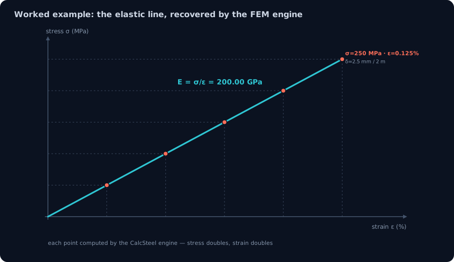
The best way to feel the first region of the curve is to actually pull a real member and watch the numbers. So we did — inside the CalcSteel. We took a real IPE 330 steel tie (cross-sectional area A = 62.61 cm²), 2 m long, in grade A36/MR250 (E = 200 GPa, fy = 250 MPa), and pulled it in pure tension with the FEM engine at five load levels. At each level we read the stress σ = N/A and the strain ε = δ/L, then divided one by the other.
Five points, one straight line
- σ = 50 MPa → ε = 0.025% → elongation δ = 0.50 mm → E = 200.00 GPa
- σ = 100 MPa → ε = 0.050% → δ = 1.00 mm → E = 200.00 GPa
- σ = 150 MPa → ε = 0.075% → δ = 1.50 mm → E = 200.00 GPa
- σ = 200 MPa → ε = 0.100% → δ = 2.00 mm → E = 200.00 GPa
- σ = 250 MPa (= fy) → ε = 0.125% → δ = 2.50 mm → E = 200.00 GPa
Look at what happens: double the stress and the strain doubles too; the 2 m bar stretches 0.50 mm, then 1.00, 1.50, 2.00, 2.50 mm in perfect proportion. The ratio σ/ε never moves — it holds at 200.00 GPa to five significant figures at every single level. That constant ratio is the straight elastic line at the start of the stress–strain curve, and its slope is Young's modulus.
σ = Eε, and what the units mean
This is Hooke's law in its engineering form: σ = Eε. Stress σ is a force per unit area, carried in MPa (N/mm²). Strain ε is a change in length divided by the original length — it is dimensionless, which is why we quote it as a percentage (0.125% is simply ε = 0.00125). Because ε carries no units, E inherits the units of stress, and for structural steel it lands around 200 GPa — the stiffness of the material.
Change the grade and the story is the same shape with a nearly identical slope — S355's E is 210 GPa versus A36's 200 GPa, a code-convention difference (ASTM ~200 / EN ~210), not a strength one. Repeating the identical experiment on S355, the engine recovered 210.00 GPa at every level from 71 MPa up to 355 MPa. Higher grade, later yield — but still a clean straight line governed by E.
One honest note on what the engine is. The CalcSteel FEM solver is a linear-elastic engine: it lives on exactly this straight line and reproduces E = σ/ε precisely, which is why the five points above are so crisp. The plastic part of the curve beyond yield is a material property that the design codes handle through the plastic modulus — and that is precisely where we go next, in the bending example (see the section on elastic vs plastic section modulus). For any point still below yield, though, the engine's answer and Hooke's law are the same answer.
Yield strength & the 0.2% offset
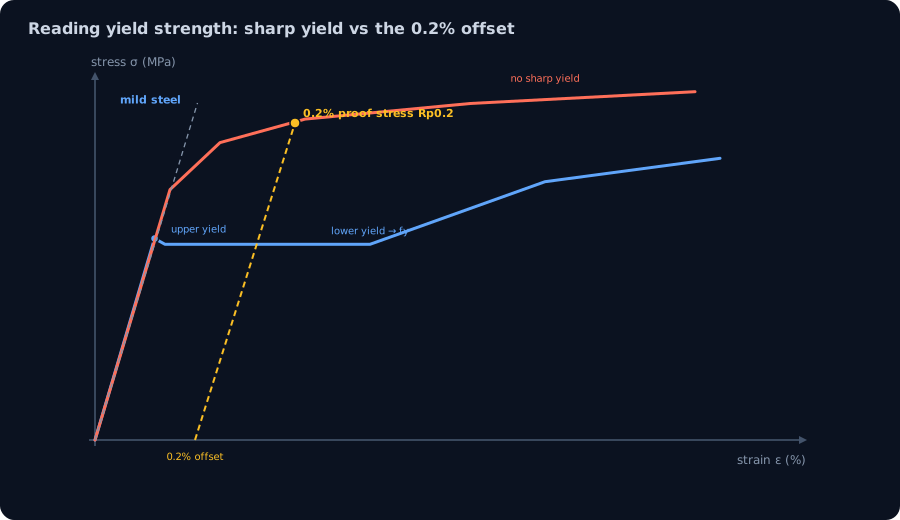
Yield strength is the stress at which elastic behaviour ends — the point where the material stops springing fully back and starts to keep some permanent deformation. On the curve it is the top of the straight elastic line, the knee. Everything below it is recoverable; everything above it is not. That single number, fy, is the value you check almost every structural design against.
Mild steel: read it straight off the curve
Hot-rolled mild steel is generous here. Its curve has a sharp upper and lower yield point followed by a flat plateau (the Lüders-band region, where slip fronts sweep through the specimen at roughly constant stress). Because the knee is so distinct, you can read fy directly — there is no ambiguity about where elastic ends and flow begins.
Rounded curves: use the 0.2% proof stress
Many materials do not give you that clean corner. Cold-formed steel, high-strength steel, stainless steel and aluminium round smoothly through the knee with no distinct yield point — the curve just bends over gradually. For these you define yield by convention using the 0.2% proof stress (Rp0.2):
- Draw a line parallel to the elastic slope (slope E).
- Offset it along the strain axis by ε = 0.2%.
- Where that offset line cuts the curve, read the stress. That stress is the proof strength — the value you then treat as fy.
The 0.2% offset is simply a repeatable agreement: it says "the stress that leaves 0.2% permanent strain behind." It lets you compare a rounded-knee material against a sharp-knee mild steel on equal terms.
Yield strain per grade, from the shipping catalog
Once you know fy and E, the strain at yield follows immediately from the elastic line: εy = fy/E. Straight from the CalcSteel material catalog:
- A36/MR250 — E = 200 GPa, fy = 250 MPa → εy = 0.125%
- S235 — E = 210 GPa, fy = 235 MPa → εy = 0.112%
- A992 (Gr.50) — E = 200 GPa, fy = 345 MPa → εy = 0.173%
- S355 — E = 210 GPa, fy = 355 MPa → εy = 0.169%
- S460 — E = 210 GPa, fy = 460 MPa → εy = 0.219%
Notice the pattern: a higher-grade steel simply reaches yield at a higher strain because it climbs further up the same straight line before turning the knee. The FEM engine confirmed the MR250 case exactly — εy = 0.00125, matching 250 MPa ÷ 200 GPa on the nose. The slope stays the same; only the height of the knee changes — a point we make sharply when we overlay every grade on one chart.
From the curve to a real stress state: the live calculator
The stress–strain curve gives you the material's limits — fy and fu — from about the simplest test there is: a single specimen pulled in one direction. But a real point buried inside a structure almost never sees a clean one-directional pull. It sees combined normal and shear stresses acting together: axial stress, bending stress and shear all landing on the same little element of steel at once.
So how do you compare that messy 2D stress state against the single yield number you read off the curve? You reduce it. Mohr's circle converts any 2D stress state into its principal stresses (the maximum and minimum normal stresses, on the planes where shear vanishes) and its maximum shear stress. Those principal values are the numbers you actually hold up against fy — the honest bridge from a laboratory pull-test to a point in a working member.
Try it right here. Feed in your σx, σy and τxy and watch the circle, the principal stresses and the maximum shear update live. It is unlimited and free, with no login for the math — drive the embedded Mohr's circle calculator below and take any stress state back to something you can compare against the curve.
σ₁ (major)
92.4MPa
σ₂ (minor)
7.6MPa
τmax in-plane
42.4MPa
θp (to σ₁)
22.5°
τabs (3-D)
46.2MPa
von Mises
88.9MPa
η · NBR
0.28 ✓
Plane-stress state (MPa)
Tension positive. τxy positive = shear that tends to rotate the element counter-clockwise on the +x face.
Plane stress (σz = 0). Enable to inspect a genuine triaxial state — three circles, not two.
Code check — steel grade
σvM = 88.9 MPa ≤ 313.6 MPa = fy / γa1 (γa1 = 1.10)
NBR 8800:2008 §5.4.2.2 (γa1 = 1,10)
From your solved model
Solve a model in the CalcSteel 3D editor, then return here to load the real σx/σy/τxy at any member section — Mohr's circle becomes the solver's inspection lens.
Presets
Element rotation θ
0°Export (free · no watermark)
Ductility, toughness & the f<sub>u</sub>/f<sub>y</sub> ratio
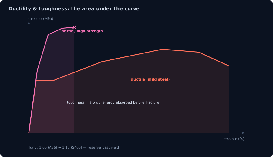
Two steels can share the same yield strength and behave completely differently once you push them past it. What separates them is ductility and toughness — the properties that decide whether a member fails with a groan and a visible sag, or snaps without warning.
Ductility is how much the material deforms before it fractures. In the tension test it is reported two ways: the elongation at fracture (percent stretch of a gauge length) and the percent reduction of area at the neck. Both measure the same thing — how far along the strain axis the curve runs before the specimen lets go. A ductile steel travels a long way to the right; a brittle one stops early.
Toughness is the area under the stress–strain curve — the energy absorbed per unit volume, in joules per cubic metre, all the way to fracture. It combines strength (how high the curve climbs) with ductility (how far it runs). This is why a long, flat yield plateau matters so much: it enlarges the area enormously for very little extra stress, and that area is the reserve a structure spends absorbing an overload, an impact or a seismic cycle without collapsing.
Resilience vs toughness
Don't confuse the two areas. The small triangle under the elastic line, up to yield, is the modulus of resilience — the energy the material stores and gives back with no permanent set. The entire area to fracture is the toughness. Elastic design lives inside the resilience triangle; ductile detailing is what lets you draw on the much larger area beyond it.
The fu/fy ratio: your reserve past yield
A single, practical number captures how much room a steel has above first yield: the ratio of ultimate strength to yield strength, fu/fy. Straight from the CalcSteel material catalog:
- A36 / MR250 — fy=250 MPa, fu=400 MPa → fu/fy = 1.60
- S235 — fy=235 MPa, fu=360 MPa → fu/fy = 1.53
- A992 (Gr.50) — fy=345 MPa, fu=450 MPa → fu/fy = 1.30
- S355 — fy=355 MPa, fu=490 MPa → fu/fy = 1.38
- S460 — fy=460 MPa, fu=540 MPa → fu/fy = 1.17
Read the table top to bottom and the trade-off is unmistakable: as the yield strength climbs from 250 MPa to 460 MPa, the reserve ratio falls from 1.60 to 1.17. Higher-strength steel yields later, but it has proportionally less headroom between the day it starts to flow and the day it breaks. That reserve is exactly what a redundant, statically indeterminate structure needs in order to redistribute load — to shed force from an overloaded fibre into neighbours before anything fractures.
Why the code polices it
EN 1993-1-1 makes this explicit, requiring structural steel to satisfy both fu/fy ≥ 1.10 and εu ≥ 15·εy. In words: the material must gain meaningful strength after yielding, and it must still be stretching many times its yield strain before it fractures. Every grade in the table above clears these limits — even S460, at 1.17, sits above the 1.10 floor — which is precisely what lets us design ductile steel structures that warn before they fail. A ductile member sags, cracks, and sheds load visibly; brittle behaviour gives none of that grace. The whole philosophy of ductile design is built on the shape of this curve, and the fu/fy ratio is its shorthand.
Steel grades on one chart: same stiffness, different strength
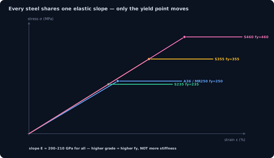
Here is the single most misunderstood fact about structural steel, and the stress–strain curve settles it in one picture. Plot A36/MR250, S235, S355 and S460 on the same axes and the elastic lines are nearly coincident — they climb from the origin at almost exactly the same slope and only peel apart when each reaches its own yield point.
That slope is Young's modulus E, and the CalcSteel catalog values say it plainly:
- A36 / MR250 — E = 200 GPa, yields at fy = 250 MPa (εy = 0.125%)
- S235 — E = 210 GPa, yields at fy = 235 MPa (εy = 0.112%)
- S355 — E = 210 GPa, yields at fy = 355 MPa (εy = 0.169%)
- S460 — E = 210 GPa, yields at fy = 460 MPa (εy = 0.219%)
Every one of these steels has E in the narrow band of 200–210 GPa. The stiffness is essentially the same across the whole family. What changes from grade to grade is where the line stops being straight — the yield point climbs from 235 MPa to 460 MPa, roughly doubling — while the slope beneath it barely moves.
Higher grade buys strength, not stiffness
State it plainly, because engineers get this wrong constantly: a higher-strength steel is not a stiffer steel. Deflection is governed by E (and by the section's moment of inertia), and E is grade-independent. Swap an S235 beam for an S460 beam of the same size (both E = 210 GPa) and it will deflect by exactly the same amount under the same load — you have only raised the stress at which it starts to yield, not the amount it sags. If your beam is failing a serviceability check, upgrading the grade does nothing; you must change the geometry, the depth or the span. See deflection limits for why this so often catches people out.
What a higher grade does buy you is a higher yield point, so a smaller section can carry the same force at the strength (ultimate) limit state — lighter, cheaper steel where strength governs. The catch, from the previous section, is that the extra strength is paid for in ductility: fu/fy falls from 1.60 for A36 down to 1.17 for S460. The line yields later, but it has less reserve once it does.
The steels that round the knee
Hot-rolled mild steel gives a sharp, unmistakable yield point. Cold-formed, high-strength quenched, and stainless steels do not — cold work and alloying round the knee into a smooth curve with no flat plateau. On the overlay chart these plot as a gently bending line with no obvious corner, which is exactly why they are read with the 0.2% proof stress from the previous section rather than an observed yield. The stiffness is still ~200–210 GPa; only the shape of the transition changes. (If you are weighing cold-formed against hot-rolled for a project, hot vs cold-formed steel unpacks the practical differences.)
The takeaway to carry away from this chart: choose a grade to win a strength argument, never a stiffness one. On a single stress–strain plot the grades share one elastic line and differ only in how high they climb before the knee.
From curve to design: elastic vs plastic section modulus
Everything so far has been about a coupon pulled in a straight line. Now watch the same curve reappear inside a beam. When a section bends, its fibres are strained in proportion to their distance from the neutral axis — so the elastic line and the plastic plateau of the stress–strain curve map directly onto how a beam yields, and onto the two section moduli you size it with.
First yield: the elastic modulus Sx
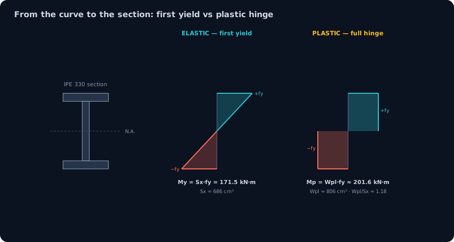
Load a beam gently and the bending stress varies linearly across the depth, peaking at the outermost fibre. Increase the moment until that extreme fibre just reaches fy — that is the exact instant the outermost point steps off the elastic line onto the knee. This is first yield, and the moment that causes it is
My = Sx · fy, where Sx is the elastic section modulus.
For an IPE 330 the CalcSteel engine gives Sx = 686 cm³, so with fy = 250 MPa:
My = 686 cm³ × 250 MPa = 171.5 kN·m.
At that moment only the top and bottom fibres are at yield; everything nearer the neutral axis is still elastic and has capacity to spare. (For a sanity check the engine ran a simply-supported IPE 330 at M = 45 kN·m and returned an extreme-fibre stress σ = M/Sx = 65.6 MPa — well below yield, and matching the hand calculation exactly.)
Full plastic hinge: the plastic modulus Wpl
Keep loading past first yield and the plastic plateau does its work: the yielded zone spreads inward from both faces while the stress at each yielded fibre holds steady at fy. When the entire section has yielded — a fully rectangular stress block, tension on one side, compression on the other — the beam forms a plastic hinge at
Mp = Wpl · fy, where Wpl is the plastic section modulus.
For the same IPE 330, Wpl ≈ 806 cm³, so:
Mp ≈ 806 cm³ × 250 MPa ≈ 201.6 kN·m.
The shape factor is the plateau, quantified
Compare the two: 201.6 vs 171.5 kN·m. The section carries about 18% more moment after first yield before it forms a hinge. That bonus is the shape factor:
Wpl / Sx ≈ 806 / 686 ≈ 1.18.
Rolled I-sections about the strong axis run roughly 1.12–1.18. This 18% is not free money — it is the plastic plateau of the stress–strain curve, cashed in at the section level. Without a ductile plateau the extreme fibre would fracture at first yield and there would be nothing to redistribute; because mild steel flows at constant stress, the inner fibres get to catch up and the whole section pulls its weight.
Which modulus you're allowed to use
You cannot always bank the shape factor. Whether a section can actually reach Mp depends on its classification — how slender its flanges and web are:
- Class 1 and 2 (compact) sections can rotate far enough to fully plasticise, so they may be designed plastically using Wpl.
- Class 3 and 4 (slender) sections buckle locally before the plateau spreads, so they are capped at first yield and limited to Sx (or an effective modulus, for Class 4).
In practice you size a beam by requiring the modulus to satisfy W ≥ M / fyd — using Wpl for a compact section, Sx for a slender one, and the design yield strength fyd. That single inequality is the stress–strain curve turned into a sizing rule. To go deeper on where these moduli come from and how axial force eats into the bending capacity, see section modulus explained and combined axial and bending, and try the numbers yourself in the moment of inertia calculator.
A real steel member on the curve
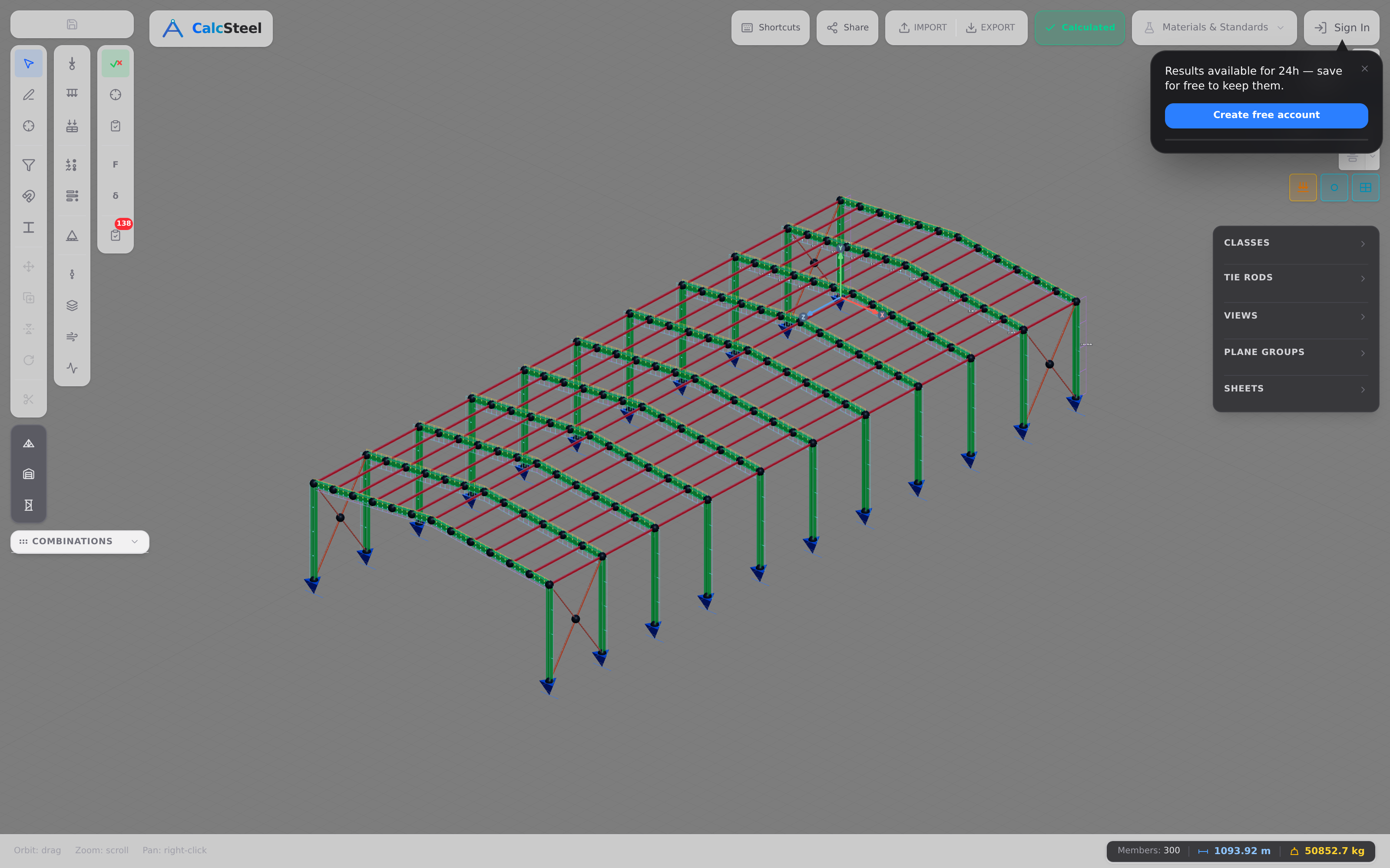
Everything so far has lived on an idealised chart. Now let's put a genuine structural member on it. We asked the CalcSteel FEM engine to solve a portal frame — 12 m span, 6 m eave columns, a 10° roof pitch, fixed bases — under gravity load on the rafters plus lateral wind. That frame is statically indeterminate, so there is no closed-form shortcut: the engine assembles the stiffness matrix and solves it, exactly the way you'd want a real design tool to.
The governing member is the IPE 330 rafter. At the critical section the engine reports a peak bending moment of 141.3 kN·m together with 23.5 kN of axial force. We turn those actions into an extreme-fibre stress by adding the bending and axial contributions:
- Bending term: σ = M / Sx = 206.0 MPa (with Sx = 686 cm³ for the IPE 330)
- Axial term: σ = N / A = 3.8 MPa
- Combined extreme-fibre stress: 206.0 + 3.8 = 209.8 MPa
Against a yield strength of fy = 250 MPa, the utilisation is σ/fy = 209.8 / 250 = 0.84. In other words, the rafter is working at 84% of yield.
Now place that on the stress–strain curve. 84% of yield sits comfortably on the elastic straight-line — well below the knee where first yield begins. The member is stiff, fully recoverable, and still holds reserve before it would even start to flow, let alone strain-harden or neck. This is precisely the operating region the codes want a primary member to live in.
Here is the part that makes the abstraction concrete: the editor's green utilisation colours are literally “where on the stress–strain curve each member sits.” A green member is on the elastic line; as utilisation climbs toward 1.0 the colour warms, telling you the extreme fibre is approaching the yield point we defined earlier in this article. The chart and the building are the same picture, drawn twice.
The combined M/Sx + N/A check here is the axial-plus-bending interaction in its simplest form; for the full unity-check story see combined axial & bending. And this is the same free, browser-native FEM engine you can drive yourself — build a frame, load it, and watch each member colour in against its own place on the curve.
Common mistakes & FAQ
The stress–strain curve is simple to draw and surprisingly easy to misread. Here are the six mistakes we see most often, followed by the long-tail questions engineers and students actually ask.
Six misconceptions to unlearn
- Confusing strength with stiffness. A higher grade does not reduce deflection. Deflection is governed by the elastic modulus E, and every structural steel shares essentially the same E ≈ 200–210 GPa. Swapping an S235 beam for an S460 beam (both E = 210 GPa) raises the yield point, but the elastic line has the same slope — the beam sags by exactly the same amount. See deflection limits.
- Blurring the proportional limit, elastic limit and yield point. The proportional limit is where σ stops being linear in ε; the elastic limit is the highest stress that still fully recovers; the yield point is where appreciable plastic flow begins. In mild steel they sit close together, which is why they get lumped — but they are three distinct definitions.
- Forgetting the 0.2% offset. Cold-formed, high-strength, stainless and aluminium alloys have a rounded knee with no sharp yield to read. You must construct the 0.2% proof stress (Rp0.2) rather than eyeballing a plateau that isn't there.
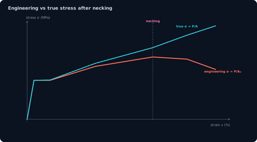
- Mixing up engineering and true stress after necking. Once a neck forms, the engineering stress (force ÷ original area) falls, so the curve dips after the UTS. The true stress (force ÷ actual, shrinking area) keeps rising to fracture. The material isn't getting weaker — the area is getting smaller.
- Assuming high-strength steel is always “better.” It yields later, but it is usually less ductile: the fu/fy ratio drops from 1.60 for A36 down to 1.17 for S460. Less reserve past yield means less warning before fracture.
- Reading fy off the curve without checking the section can reach it. The plastic moment Mp = Wpl·fy only exists if the cross-section is compact (class 1/2). A slender section buckles locally and is capped near first yield — the material's plateau is real, but the shape can't exploit it. See section modulus.
Frequently asked questions
Is Young's modulus the same for all steel? Very nearly, yes. Structural steels cluster at E ≈ 200–210 GPa regardless of grade — our FEM engine recovered exactly 200.00 GPa for A36/MR250 and 210.00 GPa for S355. Higher-strength steel is not stiffer; it simply yields at a higher stress.
What is the 0.2% proof stress? It's the practical yield strength for materials without a sharp yield point. You draw a line parallel to the elastic slope, offset by a strain of 0.2%, and read where it cuts the curve. That intersection, Rp0.2, is used as fy in design.
Why does the engineering curve go down after the UTS? Because a local neck forms and the cross-section shrinks, but engineering stress is still computed on the original area. Divide the same (or slightly falling) force by a smaller true area and the true stress is still climbing — only the bookkeeping makes the engineering curve fall.
Does higher-strength steel deflect less? No. Deflection depends on E and the section's moment of inertia, both grade-independent. Higher-strength steel lets you carry more load before yielding, but at the same load and section it deflects the same amount.
Key takeaways
Walk away with these five points and you can read any steel stress–strain curve — and know what it means for a real structure.
- The curve is the material's fingerprint. One tension test fixes E (stiffness), fy (yield), fu (ultimate strength) and ductility all at once, across five regions: elastic line, yield, strain hardening, necking, fracture.
- The elastic line is Hooke's law, and the engine lives on it. σ = Eε with E recovered to 200.00 GPa (A36) and 210.00 GPa (S355) at every load level — a linear-elastic FEM solver reproduces the straight line exactly.
- Same stiffness, different strength. Every structural steel shares E ≈ 200–210 GPa; a higher grade buys a higher yield point, not less deflection — and usually costs you ductility (fu/fy falls from 1.60 to 1.17).
- The plateau is design capacity. First yield My = Sx·fy = 171.5 kN·m; the full plastic hinge Mp = Wpl·fy ≈ 201.6 kN·m for an IPE 330 — about 18% more, thanks to the plastic plateau of the curve.
- Real members sit somewhere on the curve. The portal-frame rafter at σ = 209.8 MPa, utilisation 0.84, is on the elastic straight-line below the knee — and the editor's green colours show you exactly that, member by member.
Try it yourself — free
The curve gives the limits; a real stress state gives the numbers. Drive the Mohr's circle calculator to turn any 2D stress state into its principal stresses and maximum shear — unlimited and free, no login for the math. Then build the whole structure in the CalcSteel, a genuinely-free, browser-native steel design & analysis solution with a real FEM engine, and watch each member colour in against its own place on the stress–strain curve.
Students and labs: the proof is in your hands. CalcSteel /education is free for students and research labs at any university — the same engine, the same curve, no barrier.
Sources
Try CalcSteel for free
Model, analyze and design steel structures in your browser. No install, no signup.
Open the 3D editor