Strain Rosettes: Reading a Real Gauge on a Loaded Steel Member

A strain gauge measures one number: the normal strain along its own axis. A loaded steel member has three unknowns at every point on its surface. This guide shows how three gauges in a rosette recover the full strain state, how the 45 degree and 60 degree layouts differ, and how to turn three microstrain readings into principal stresses and a von Mises number, with every value checked against the CalcSteel FEM engine on a real IPE 300 beam.
Key takeaways
- A single strain gauge reads only the normal strain along its own grid. The surface of a loaded member has three unknowns, εx, εy and γxy, so you need three gauges at three angles. That set of three is a strain rosette.
- The transformation law ε(θ) = εx cos²θ + εy sin²θ + γxy sinθ cosθ is the whole subject. Invert it for the two standard layouts: rectangular 0/45/90 gives γxy = 2εb − εa − εc directly; delta 0/60/120 gives εy = (2εb + 2εc − εa)/3 and γxy = 2(εb − εc)/√3.
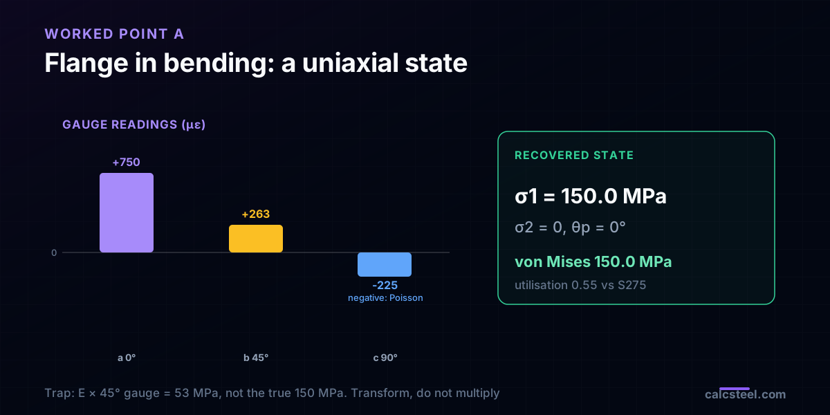
- On the midspan bottom flange of the worked IPE 300, the state is uniaxial: the gauges read +750, +263 and −225 µε. The 90 degree gauge reads negative from Poisson, and reading E times the 45 degree gauge would report 53 MPa instead of the true 150 MPa. You must transform, not multiply.
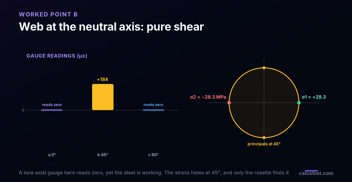
- On the web at the neutral axis over the support, the state is pure shear: the axial and transverse gauges read exactly zero while the 45 degree gauge reads +184 µε. A single axial gauge there says the steel is unloaded, yet the principal stresses are ±28 MPa. This is why a rosette is mandatory when you do not know the principal directions.
- Once you have εx, εy and γxy, plane stress Hooke's law gives the principal stresses σ1,2 = E/(1−ν²)(ε1 + ν ε2) and the von Mises stress that the code checks against yield. The rosette round trip on all three points reproduced the beam theory value to the third decimal.
What does a gauge on a loaded beam actually tell you?
Bond a foil strain gauge to the flange of a loaded steel beam, read the bridge, and you get one number: microstrain along the direction the grid happens to point. That number feels like an answer, but on its own it is almost useless for stress. The steel at that point is in a two dimensional state, and one reading cannot separate how much of the strain is stretching along the member, how much is the Poisson squeeze across it, and how much is shear sliding the surface. Three quantities, one measurement.
The fix is old, cheap and everywhere in a test lab: put three gauges at three known angles at the same point and read all three. That cluster is a strain rosette. With three readings you can solve for the three unknowns of the surface strain state, rotate to the principal directions, and only then convert to stress. This is the bridge between what an instrument can measure, strain, and what a code checks, stress.
This guide is written for three readers at once. If you are a student meeting rosettes in a mechanics of materials course, this is the chapter that usually collapses into one dense slide of trigonometry. If you are a practising engineer or a freelance calculista validating a model against a physical test, this is how you turn the data logger into a stress you can compare with your analysis. And if you just want the punchline: on a loaded member you rarely know the principal directions in advance, so one gauge can read zero where the stress is highest.
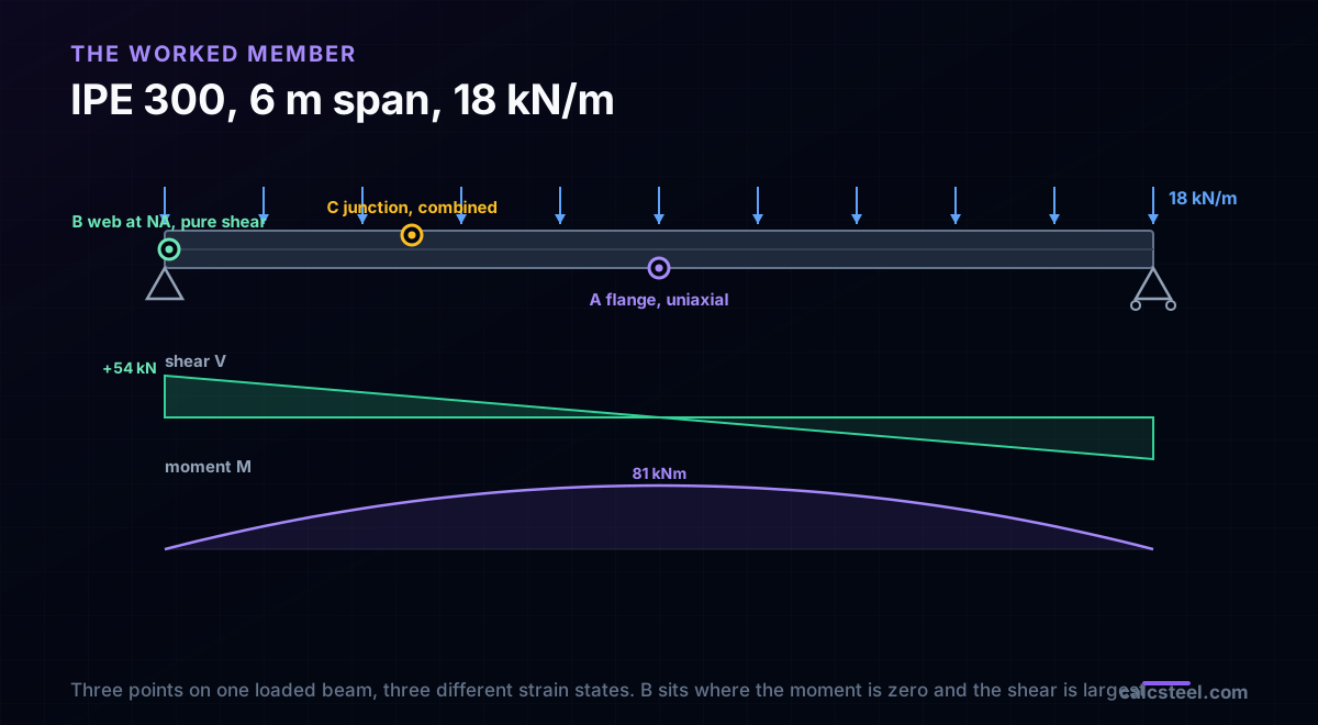
Every number in the worked examples came from the CalcSteel FEM engine running a real IPE 300 beam, then the beam theory stresses were fed through the rosette maths and inverted back. The loop closed to three decimals, which is the point of the whole exercise: the gauge reads what the analysis predicts, once you do the transformation correctly.
One gauge, three unknowns, and why three readings
The surface of a loaded member is a plane stress problem: the free face carries no stress through its thickness, so the state at a point is fully described by three numbers in the surface plane. In strain terms those are the normal strain along the member axis εx, the normal strain across it εy, and the engineering shear strain γxy, the change in the right angle between those two directions.
A strain gauge does not measure any of these directly unless you happen to align it perfectly. It measures the normal strain along its own grid, at whatever angle θ that grid sits. The transformation law connects the two:
ε(θ) = εx cos²θ + εy sin²θ + γxy sinθ cosθ
One gauge gives one equation in three unknowns. Two gauges give two equations, still short. Three gauges at three distinct angles give three independent equations, and now the system is solvable for εx, εy and γxy. That is the entire reason a rosette has three grids and not two or four. A fourth gauge is sometimes added only as a redundant check, never because the maths needs it.
Notice what this means physically. If you guess the member is in simple tension and glue one gauge along the axis, you are betting that εy and γxy do not matter to you. On a flange in pure bending that bet happens to pay off. On a web in shear it fails completely, as the worked example below shows, and there is no warning in the single reading that tells you the bet was wrong.
The two rosettes you will actually meet: 45 and 60 degrees
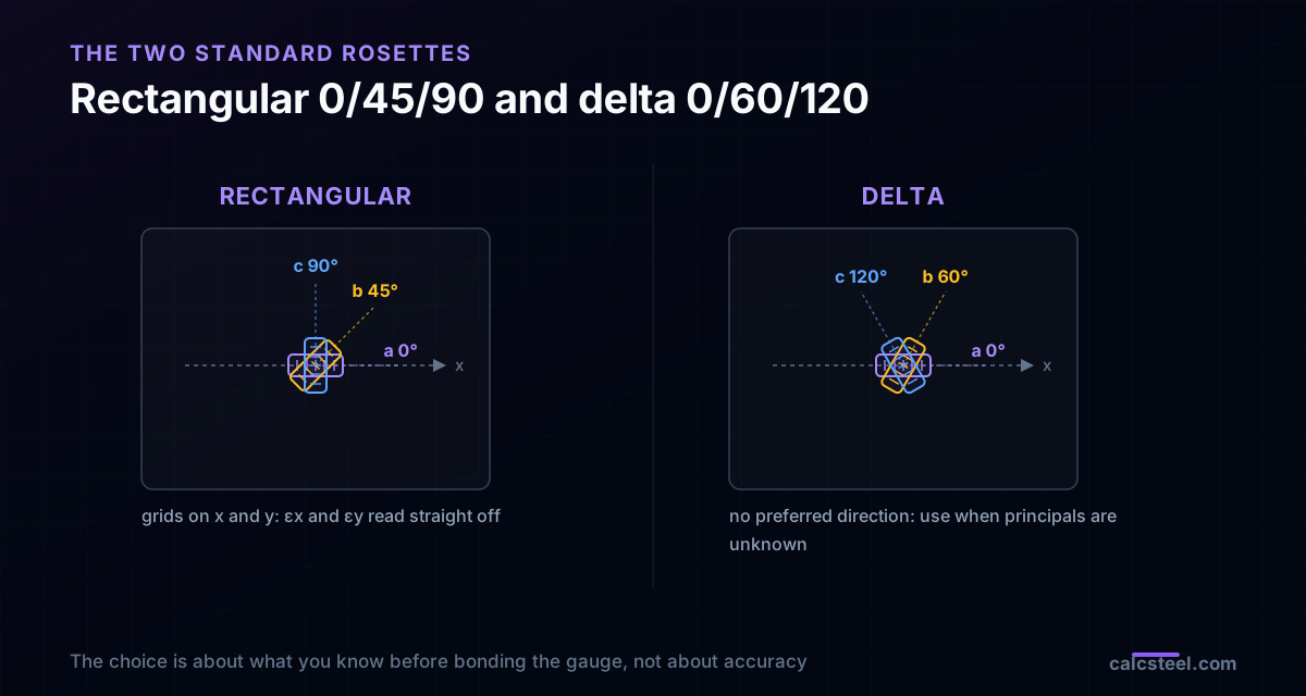
Any three distinct angles work in principle, but manufacturers standardise two layouts because their inversion formulas are clean and their errors are well behaved.
The rectangular rosette, 0 / 45 / 90
Three grids at 0, 45 and 90 degrees. It is the workhorse. Because gauge a sits on the x axis and gauge c on the y axis, two of the three unknowns fall out with no algebra at all: εx = εa and εy = εc. Only the shear needs the 45 degree reading. Use it when you have a sensible guess at the principal directions, for example a gauge lined up with the axis of a beam or a column, because then gauge a and gauge c land near the principal values.
The delta rosette, 0 / 60 / 120
Three grids at 0, 60 and 120 degrees, spread evenly around the circle. It has no preferred direction, so it is the honest choice when the principal directions are genuinely unknown, near a weld, a hole, a bracket, or a region of combined load. The inversion needs a little more arithmetic, but it is symmetric and numerically well conditioned.
Both come as tight stacked patterns a few millimetres across so all three grids sample essentially the same point. The choice between them is about what you know before you bond the gauge, not about accuracy. Get the wiring order and the reference direction of gauge a recorded on the test sheet, because every formula that follows depends on which physical grid you call a, b and c.
The transformation law, term by term
Everything in this article is one equation applied three times. It deserves a careful read, because the single most common rosette error hides inside it.
ε(θ) = εx cos²θ + εy sin²θ + γxy sinθ cosθ
- εx cos²θ projects the axial normal strain onto the gauge direction. At θ = 0 it is all of εx; at θ = 90 it vanishes.
- εy sin²θ does the same for the transverse normal strain. At θ = 90 it is all of εy.
- γxy sinθ cosθ is the shear contribution. It is zero at θ = 0 and θ = 90, and largest at θ = 45. This is why the 45 degree gauge is the one that senses shear.
The trap is the definition of γxy. This formula uses the engineering shear strain, the full change of the right angle. The tensor shear strain used in Mohr's circle is half of it, εxy = γxy / 2. Mix the two and every shear result is out by a factor of two, silently, because both numbers look plausible. Throughout this guide γ is engineering shear strain, and the factor of one half appears explicitly wherever the circle needs it.
One more habit worth keeping: strains here are quoted in microstrain, µε, meaning parts per million, 10⁻⁶. A reading of 750 µε is a strain of 0.000750. Steel yields at roughly 1250 to 1750 µε depending on grade, so a rosette on a working member lives in the few hundred µε range, which is exactly what the examples show.
Solving the rectangular rosette
Write the transformation law at the three angles of the 0/45/90 rosette and the algebra almost disappears.
At θ = 0: εa = εx.
At θ = 90: εc = εy.
At θ = 45: εb = εx (½) + εy (½) + γxy (½) = (εx + εy)/2 + γxy/2.
The first two give εx and εy for free. Rearrange the third for the shear:
γxy = 2εb − εa − εc
That is the entire inversion. Three readings in, three strain components out, with a subtraction. The reason the 45 degree gauge cannot be dropped is now obvious: without εb there is no way to reach γxy, and γxy is what carries all the shear information.
A quick sanity check you can run on any dataset: if 2εb equals εa + εc, the shear is zero and your gauge axes are already the principal axes. If it does not, the difference is the shear, and the principal directions are rotated away from your gauge lines.
Solving the delta rosette
The delta rosette spreads its grids at 0, 60 and 120 degrees. Gauge a still lands on the x axis, so εx = εa as before. The other two need the transformation law with cos²60 = ¼, sin²60 = ¾, and sinθ cosθ = ±√3/4:
εb = ¼ εx + ¾ εy + (√3/4) γxy
εc = ¼ εx + ¾ εy − (√3/4) γxy
Add the two to cancel the shear, then solve for εy; subtract them to isolate γxy:
εy = (2εb + 2εc − εa) / 3
γxy = 2(εb − εc) / √3
The symmetry is the whole appeal. The transverse strain comes from the sum of the two off axis gauges, the shear from their difference, and neither formula favours any direction. That even handedness is why the delta layout is the right tool near a weld toe or a bracket, where you have no honest guess at where the principal axes point.
From strain components to principal strains and direction
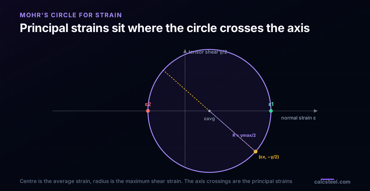
With εx, εy and γxy in hand, the surface strain state is fully known, and finding its principal values is the same Mohr's circle you already use for stress, with the tensor shear εxy = γxy/2 on the vertical axis. The principal strains are:
ε1,2 = (εx + εy)/2 ± √[ ((εx − εy)/2)² + (γxy/2)² ]
and the angle from the x axis to the ε1 direction is:
tan 2θp = γxy / (εx − εy)
The centre of the circle is the average normal strain, and its radius is the largest shear strain the point sees, γmax/2. The two principal strains are the extreme normal strains, and they act on planes free of shear. For steel, where the surface is unyielded and elastic, these principal strains map straight onto principal stresses in the next step.
You can feel the whole construction by moving the shear slider in the Mohr's circle tool below and watching the principal angle swing. When γxy is zero the circle sits on the horizontal axis and the principal directions are your gauge lines. As shear grows the circle lifts and the principal axes rotate toward 45 degrees, which is exactly the pure shear case the web gauge will show.
The step everyone wants: strain to stress
A rosette measures strain, but design is written in stress. The elastic surface is in plane stress, so the two principal stresses come from the two principal strains through Hooke's law:
σ1 = E/(1 − ν²) · (ε1 + ν ε2)
σ2 = E/(1 − ν²) · (ε2 + ν ε1)
with steel E = 200 GPa and ν = 0.30. The coupling term ν ε2 matters: you cannot convert each principal strain to a stress on its own, because a strain in one direction produces stress in both through Poisson's effect. Skip the coupling and a uniaxial flange with ε2 = −225 µε would report a spurious 45 MPa on the second axis instead of zero.
Once you have the principal stresses, the number a steel code actually checks is the von Mises equivalent stress, which for a plane stress state is:
σvm = √(σ1² − σ1σ2 + σ2²)
Compare σvm with the yield stress, 275 MPa for the S275 steel in the example, and you have a utilisation. This is the same criterion behind the code checks in the Mohr circle and principal stress guide, reached here from a physical measurement instead of a computed stress. The three worked points below run this pipeline end to end.
Worked point A: the flange in bending, a uniaxial state
Take the IPE 300 over a 6 m span under a uniform 18 kN/m. The CalcSteel engine returns a midspan moment of 81.0 kNm with zero shear there, matching wL²/8 exactly. Bond a rectangular rosette to the bottom flange at midspan, gauge a along the member axis. The section modulus the engine uses for this shape is Sx = 540 cm³, so the fibre stress is:
σx = M / Sx = 81.0 kNm / 540 cm³ = 150.0 MPa tension, with σy = 0 and τ = 0.
This is a uniaxial state, so the strains are εx = σx/E = 750 µε and εy = −ν εx = −225 µε. Feed them through the transformation law and the three gauges read:
- Gauge a, 0 degrees: +750.3 µε, the full axial stretch.
- Gauge b, 45 degrees: +262.6 µε, the average of the two normal strains, (750.3 − 225.1)/2.
- Gauge c, 90 degrees: −225.1 µε, the Poisson contraction across the flange, and it is negative.
Invert: γxy = 2(262.6) − 750.3 − (−225.1) = 0, so the gauge axes are principal, θp = 0. The principal strains are just εa and εc, and Hooke's law gives σ1 = 150.0 MPa, σ2 = 0, von Mises 150.0 MPa, a utilisation of 0.55 against S275.
Two lessons live in this simple point. First, the 90 degree gauge reads negative even though the flange is in tension, purely from Poisson, and a reader who forgets that will think the flange is in compression across its width. Second, the trap: if you had bonded a single gauge and it happened to sit at 45 degrees, you would read 262.6 µε and, multiplying by E, report 53 MPa. The true stress is 150 MPa. The gauge is not wrong. Reading it as if it were aligned is wrong.
Worked point B: the web over the support, pure shear
Now move the gauge to the web at the neutral axis, directly over the support. Here the engine returns the maximum shear, V = 54 kN, equal to wL/2, and the bending moment is zero. At the neutral axis the bending stress is zero by definition, so the state is pure shear. The shear stress from the beam is τ = VQ/(I t), with the engine's first moment Q = 301 × 10³ mm³, second moment I = 8097 cm⁴ and web thickness t = 7.1 mm:
τ = (54 kN)(301 × 10³ mm³) / (8097 cm⁴ × 7.1 mm) = 28.3 MPa, with σx = σy = 0.
Pure shear means εx = 0 and εy = 0, and only γxy = τ/G = 368 µε is non zero. Put a rectangular rosette here, gauge a along the axis, and the readings are stark:
- Gauge a, 0 degrees: 0 µε.
- Gauge b, 45 degrees: +183.8 µε, which is γxy/2.
- Gauge c, 90 degrees: 0 µε.
Invert: γxy = 2(183.8) − 0 − 0 = 367.6 µε. The principal strains are ±183.8 µε at θp = 45 degrees, and Hooke's law gives principal stresses of +28.3 and −28.3 MPa, a von Mises of 49.0 MPa.
This is the example that justifies the whole instrument. A single gauge bonded along the member axis at this point reads exactly zero and tells you the steel is unloaded. It is not: the principal stresses are ±28 MPa and the material is working. The stress hides at 45 degrees, where no axial gauge is looking, and only the rosette finds it. Whenever you cannot promise where the principal directions lie, one gauge can read zero at the worst point.
Worked point C: the web-flange junction, a combined state
The most general point carries bending and shear together, and its principal directions land at neither 0 nor 45 degrees. Take the junction of web and flange at the quarter span, x = 1.5 m, on the compression side. The engine returns M = 60.75 kNm and V = 27 kN there. At the junction, y = 139.3 mm from the neutral axis, the bending stress is σx = −M y / I = −104.5 MPa (compression), and the shear from the flange first moment Q = 232 × 10³ mm³ is τ = 10.9 MPa.
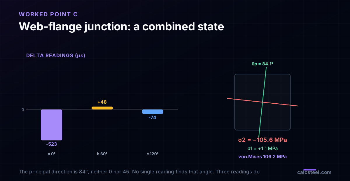
Because the principal directions are unknown here, use a delta rosette, gauge a along the axis. The plane stress strains are εx = (σx − ν σy)/E = −522.6 µε, εy = −ν σx/E = +156.8 µε, and γxy = τ/G = 141.7 µε. The three delta gauges read:
- Gauge a, 0 degrees: −522.6 µε.
- Gauge b, 60 degrees: +48.3 µε.
- Gauge c, 120 degrees: −74.4 µε.
Invert with the delta formulas: εx = −522.6, εy = (2·48.3 + 2·(−74.4) − (−522.6))/3 = +156.8 µε, and γxy = 2(48.3 − (−74.4))/√3 = +141.7 µε. The principal strains are +164.1 and −529.9 µε at θp = 84.1 degrees, a direction you would never have guessed. Hooke's law gives principal stresses σ1 = +1.1 MPa and σ2 = −105.6 MPa, and a von Mises of 106.2 MPa, a utilisation of 0.39 against S275.
The takeaway is the rotated principal axis. The dominant action is axial compression, so the principal compression sits near the member axis and the principal tension near vertical, at 84 degrees. No two gauge cluster and no single reading would have found that angle. Only three readings, run through the transformation, recover both the magnitude and the direction.
Six mistakes that quietly corrupt a rosette result
Each of these turns clean gauge data into a wrong stress, and none of them throws an error at the data logger.
- Engineering versus tensor shear. The transformation law uses engineering γxy, Mohr's circle uses γxy/2. Feed γxy into the circle as if it were the tensor value and every shear result doubles.
- Losing the gauge order. Every formula depends on which physical grid is a, b and c and which way gauge a points. Swap b and c on a delta rosette and the shear sign flips, rotating the principal axis the wrong way. Record the reference direction on the test sheet.
- Multiplying a single reading by E. E times a gauge reading is a stress only if that gauge is aligned with a principal axis and the state is uniaxial. On the 45 degree gauge or on a sheared web it gives a confident wrong number.
- Dropping the Poisson coupling. σ1 depends on both ε1 and ε2 through E/(1−ν²)(ε1 + ν ε2). Converting each principal strain alone overstates one axis and invents stress on the other.
- Ignoring temperature. A bonded gauge responds to thermal expansion as well as load. Without a dummy gauge or self temperature compensated foil, a few degrees of drift reads as tens of microstrain of phantom load.
- Forgetting it is a surface measurement. A rosette reads the free surface, where the through thickness stress is zero. That is plane stress, which is what the Hooke's law form above assumes. It is not the interior of the section, and it is not plane strain.
Try it live, and know what the gauge should read
The fastest way to internalise the strain circle is to move it. The calculator below is the CalcSteel Mohr's circle tool, free and with no login for the maths. Enter the recovered εx, εy and γxy from any of the worked points, or type a stress state directly, and watch the principal values and the rotation angle update. Put in the pure shear web, εx = εy = 0 with γxy = 368 µε, and see the circle centre on the origin with principal directions at 45 degrees.
In practice the workflow runs both ways. Before a test, you build the member in CalcSteel, read the moment and shear at the gauge location from the FEM engine, and compute the strain the rosette should read, so an outlier on the day flags a debond or a wiring error rather than a surprise in the steel. After a test, you invert the real readings through the formulas here and compare the von Mises stress with the analysis. The three points above were generated exactly this way, engine forces out, rosette maths in, and the loop closed to three decimals.
From here, the two neighbours worth reading are the Mohr's circle construction that underlies the principal step, and yield strain, which sets the microstrain level where the elastic Hooke's law you used here stops being valid.
σ₁ (major)
92.4MPa
σ₂ (minor)
7.6MPa
τmax in-plane
42.4MPa
θp (to σ₁)
22.5°
τabs (3-D)
46.2MPa
von Mises
88.9MPa
η · NBR
0.28 ✓
Plane-stress state (MPa)
Tension positive. τxy positive = shear that tends to rotate the element counter-clockwise on the +x face.
Plane stress (σz = 0). Enable to inspect a genuine triaxial state — three circles, not two.
Code check — steel grade
σvM = 88.9 MPa ≤ 313.6 MPa = fy / γa1 (γa1 = 1.10)
NBR 8800:2008 §5.4.2.2 (γa1 = 1,10)
From your solved model
Solve a model in the CalcSteel 3D editor, then return here to load the real σx/σy/τxy at any member section — Mohr's circle becomes the solver's inspection lens.
Presets
Element rotation θ
0°Export (free · no watermark)
Sources
- 1.Hibbeler, Mechanics of Materials, chapter on strain transformation (strain rosettes, Mohr's circle for strain)
- 2.Boresi and Schmidt, Advanced Mechanics of Materials, strain gauge rosette analysis
- 3.Vishay Micro-Measurements, Tech Note TN-515, Strain Gage Rosettes: Selection, Application and Data Reduction
- 4.ASTM E251, Standard Test Methods for Performance Characteristics of Metallic Bonded Resistance Strain Gauges
Try CalcSteel for free
Model, analyze and design steel structures in your browser. No install, no signup.
Open the 3D editor