Residual Stresses in Rolled Shapes: Why the Column Curve Is Not the Euler Curve

Euler says a pinned W 250 x 73 buckling about its weak axis at 5 m carries 3063 kN. Yielding says the same bar cannot exceed 3172 kN. Both numbers are right, and the code still answers 2056 kN. A third of the capacity is gone, and no safety factor has been applied yet. The missing third is residual stress: locked-in stress that the rolling mill put into the steel while it cooled, before any load was ever applied. This article follows that stress from the cooling bed to the buckling curve, with every number computed by the CalcSteel FEM engine and checked against closed form.
Key takeaways
- A rolled shape cools unevenly. Flange tips and mid web cool first and set; the web-to-flange junction cools last, and its shrinkage is resisted by metal that is already rigid. The result is compression at the flange tips and tension at the junction, with no load applied.
- The ECCS model puts the peak at 0.5 fy for shapes with h/b ≤ 1.2 and 0.3 fy for h/b > 1.2. On a W 250 x 73 in 345 MPa steel that is 172.5 MPa already sitting in the flange tips.
- Residual stress is self-equilibrating, so it does not change the squash load, and it disappears into the elastic buckling load of a very slender column. It bites hardest in between: at λ₀ = 1.0 the code keeps only 0.658 of what Euler and yielding together would promise, a 34.2 % loss.
- The tips yield first, and the tips are exactly the material with the longest lever arm about the weak axis. With 30 % of the flange width yielded, the strong-axis stiffness keeps 72.2 % but the weak-axis stiffness keeps only 34.3 %. That asymmetry is why EN 1993 sends this shape to curve b about y-y and curve c about z-z.
- The numbers in AISC 360 carry the history: 0.658 and 0.877 are calibration coefficients fitted at λ = 1.0 and λ = 1.5, and the λ = 1.5 crossover was chosen to preserve the older ASD match at Fy/2, which is the 0.5 fy residual-stress assumption written into the CRC parabola.
The third of the capacity that Euler never mentions
Take a W 250 x 73, ASTM A572 Grade 50, fy = 345 MPa, pinned at both ends, 5 m long, buckling about its weak axis. Two textbook answers bracket the problem. Euler gives the elastic critical load, Ncr = π²EI/L² = 3063 kN. Yielding gives the squash load, A·fy = 3172 kN. The column cannot beat either one, so the honest ceiling is the lower of the two: 3063 kN.
Now ask the engine. Running the same bar through the shipping CalcSteel check, AISC 360 Chapter E returns a nominal strength of 2056 kN, and NBR 8800 returns the same 2056 kN before its partial factor. That is 32.9 % below the ceiling the two classical formulas set, and no resistance factor has been applied yet. The φ and the γ come afterwards, and they take more.
That gap is not conservatism, and it is not a fudge. It is a measured physical effect that has its own name: residual stress. The bar arrived at the site already stressed. Nobody loaded it. The rolling mill did it, and it happened while the steel was cooling on the bed, in the hours after it left the last stand.
This article follows that stress from where it is created to where it shows up in your design check: the cooling order of a hot section, the pattern it leaves behind, why the pattern attacks the weak axis harder than the strong one, and how it turned the Euler hyperbola into the column curve that every modern code actually uses.
Where they come from: a shape that does not cool all at once
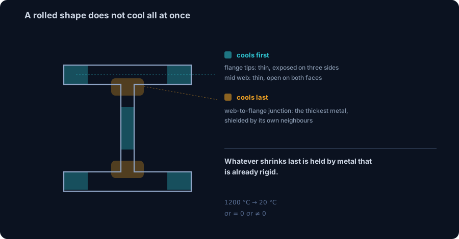
A hot-rolled section leaves the last rolling stand at roughly 1000 °C and cools in still air. If every fibre cooled at the same rate, the shape would shrink uniformly and finish with zero internal stress. It does not, for a reason that is entirely geometric.
Cooling rate depends on how much surface a piece of metal has relative to its volume, and on how much hot neighbouring metal is radiating back at it. On an I section those two things vary a lot from point to point:
- The flange tips are thin, and they are exposed on three sides at once. They lose heat fastest.
- The middle of the web is thin and open on both faces. It also cools fast.
- The web-to-flange junction is the thickest metal in the section, and it is surrounded on every side by other hot metal that keeps radiating at it. It cools last, often by a wide margin.
Here is the mechanism, and it is worth stating slowly because everything downstream follows from it. The tips cool first, contract, and become rigid while the junction is still soft and hot. Then the junction cools and tries to contract in turn. But it is now attached to metal that has already set. Its shrinkage is resisted.
A region that wants to shrink and is held ends up in tension. The regions holding it must push back, so they end up in compression. The steel reaches room temperature with a locked-in stress field it can never shed: tension where it cooled last, compression where it cooled first. No load has been applied, and the bar is already stressed to a level that matters.
The pattern, and the number that goes with it
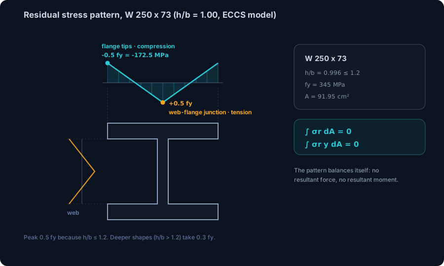
Measured residual stress patterns in hot-rolled I sections are remarkably consistent, which is why they could be turned into a design model. The ECCS pattern, the one behind the European buckling curves, describes a hot-rolled I shape like this:
- Compression at the flange tips, falling linearly across the flange.
- Tension at the web-to-flange junction and through the flange centre.
- Tension in the web near the flanges, turning to compression at mid-height.
The magnitude depends on the proportions of the shape, and the split is at h/b = 1.2:
| Shape | Peak residual stress | In 345 MPa steel |
|---|---|---|
| h/b > 1.2 (deep and narrow: IPE, most beam shapes) | 0.3 fy | 103.5 MPa |
| h/b ≤ 1.2 (stocky and wide: HEB, W column shapes) | 0.5 fy | 172.5 MPa |
Our W 250 x 73 is 253 mm deep and 254 mm wide, so h/b = 0.996 and it falls on the severe side. Before anyone loads it, its flange tips are carrying about 172.5 MPa of compression. That is half the yield stress of the material, spent.
Two properties of this stress field decide everything that follows. First, it is self-equilibrating: integrate it over the cross-section and you get zero force and zero moment. It has to, because nothing external is holding the bar. Second, it is not uniform: it is compression in exactly the places that matter most for stability.
The self-equilibrium is what makes residual stress so easy to dismiss. A very stocky column, one too short to buckle at all, still reaches A·fy. The compressed tips yield early, the tensioned centre picks up the difference, and the total squash load is unchanged. Residual stress costs nothing there. It is when the column has to stay straight that the bill arrives.
Load it, and the applied stress lands on top of what is already there
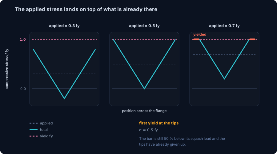
Now push on the column. The applied compression is uniform across the section, at least while everything is elastic. It does not replace the residual stress; it adds to it. What each fibre feels is the sum.
Follow the flange tips, which are already at 0.5 fy in compression. They reach yield when
σapplied + 0.5 fy = fy, so σapplied = 0.5 fy = 172.5 MPa
The column starts yielding at half of its squash load. Not at 90 %, not at 100 %. At 50 %, in the flange tips, while the rest of the section is comfortably elastic and while the average stress on the bar still looks entirely safe on paper.
Push further and the yielded zone spreads inward from the tips. At an applied 0.7 fy, the outer 10 % of each flange half has gone plastic. The bar is not failing, and a stress check would not complain. But something has changed that a stress check cannot see: the yielded metal no longer contributes stiffness. Yielded steel has a tangent modulus near zero. For the purpose of resisting the next increment of bending, those tips have stopped existing.
This is the hinge of the whole subject. Buckling is a stiffness problem, not a strength problem. A column buckles when the bending stiffness it can still mobilise stops being enough to restore it against the load trying to bend it. Residual stress does not reduce the material strength anywhere. It reduces the stiffness available at the moment of buckling, by yielding parts of the section early.
Why the weak axis pays the most
Here is the part that is rarely spelled out, and it explains a curiosity every student runs into: why do the codes treat the two axes of the same rolled shape differently, when the residual stress pattern is identical for both?
Because of where the yielding happens. The first metal to go plastic is the flange tips, and the flange tips are the material with the longest lever arm about the weak axis. About the strong axis they contribute through their distance from the neutral axis in the depth direction, which is the same for the whole flange width. About the weak axis they contribute through their distance across the flange width, and losing the outermost band is expensive.
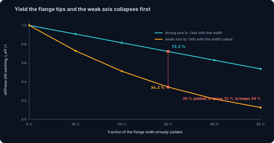
Put numbers on it. If a band of width c yields at each tip, the elastic core of each flange has width be = b − 2c, and:
- Strong axis: Ix of the flanges is roughly be·tf·(h/2)², proportional to be. Lose 30 % of the width and you lose about 30 % of the flange term.
- Weak axis: Iy of the flanges is tf·be³/12, proportional to becubed. Lose 30 % of the width and you keep 0.7³ = 34 % of the flange term.
Computed on the real W 250 x 73 geometry, web included:
| Flange width yielded | Ix still working | Iy still working |
|---|---|---|
| 0 % | 100 % | 100 % |
| 10 % | 90.7 % | 72.9 % |
| 20 % | 81.5 % | 51.2 % |
| 30 % | 72.2 % | 34.3 % |
| 50 % | 53.7 % | 12.5 % |
At 30 % yielded, the strong axis has lost about a quarter of its stiffness and the weak axis has lost two thirds. Same section, same residual stress, same applied load. The difference is purely which axis the lost material was working for.
That single asymmetry is why EN 1993-1-1 does not give a rolled I section one buckling curve. It gives it two, one per axis, and the weak axis always gets the worse one.
From the Euler hyperbola to the column curve
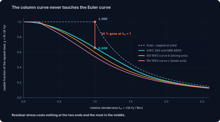
Classical column theory offers two limits and nothing in between. Euler gives the elastic critical stress, valid for slender members. Yielding gives fy, valid for stocky members. Plot both against relative slenderness λ₀ = √(A·fy/Ncr) and you get a flat line at χ = 1 up to λ₀ = 1, then the Euler hyperbola χ = 1/λ₀². They meet in a corner at λ₀ = 1.
Real columns do not follow that corner. They fall well below it, and the tests have been saying so since the nineteenth century. Residual stress is the main reason, initial out-of-straightness is the other, and the two interact: a bar that is slightly bent and has yielded tips is far weaker than either effect alone would suggest.
Sweeping λ₀ from 0.01 to 2.6 and comparing the AISC 360 curve against the Euler-and-yield ceiling, the loss is not uniform. It has a clear maximum:
| λ₀ | Euler capped at yield | AISC 360 and NBR 8800 | Lost |
|---|---|---|---|
| 0.2 | 1.000 | 0.974 | 2.6 % |
| 0.5 | 1.000 | 0.901 | 9.9 % |
| 1.0 | 1.000 | 0.658 | 34.2 % |
| 1.5 | 0.444 | 0.390 | 12.3 % |
| 2.0 | 0.250 | 0.219 | 12.3 % |
| 2.5 | 0.160 | 0.140 | 12.3 % |
The worst point is λ₀ = 1.0, where the code keeps 0.658 of the classical ceiling and throws away 34.2 %. That is not a coincidence of the plot: 0.658 raised to the power λ₀² is exactly the AISC inelastic formula, and at λ₀ = 1 the exponent is 1, so the coefficient shows up undisguised.
Look at the two ends and the shape of the effect becomes obvious. For a very stocky column, residual stress is self-equilibrating and the squash load is untouched. For a very slender column, buckling happens at a stress so low that nothing has yielded, so the full elastic stiffness is available and only the out-of-straightness allowance remains, the flat 12.3 % you see in the tail. In between, partial yielding is at its most damaging, and that is precisely where most real columns live.
Residual stress costs nothing at the two ends and the most in the middle. If you remember one sentence from this article, that is the one.
The W 250 x 73 through the real engine
Enough theory. Below is the same shape run through the shipping CalcSteel design check at a range of lengths, pinned, buckling about the weak axis. Every engine value was reproduced by hand from the code equations before it was published, 68 checks in total, and the run aborts if any pair disagrees by more than 0.02 %.
The section as the engine computes it from the rolled geometry: A = 91.95 cm², Ix = 11124 cm⁴, Iy = 3880 cm⁴, rx = 11.00 cm, ry = 6.50 cm. Against the published catalogue values that is 1.0 % low on area and 0.2 % low on Iy, the usual difference from how the root fillets are idealised. Squash load A·fy = 3172 kN.
| Length | λ = L/ry | λ₀ | Euler Ncr | Classical ceiling | AISC 360 Pn | Lost |
|---|---|---|---|---|---|---|
| 2 m | 30.8 | 0.407 | 19145 kN | 3172 kN | 2960 kN | 6.7 % |
| 3 m | 46.2 | 0.611 | 8509 kN | 3172 kN | 2714 kN | 14.4 % |
| 4 m | 61.6 | 0.814 | 4786 kN | 3172 kN | 2404 kN | 24.2 % |
| 5 m | 77.0 | 1.018 | 3063 kN | 3063 kN | 2056 kN | 32.9 % |
| 6 m | 92.4 | 1.221 | 2127 kN | 2127 kN | 1699 kN | 20.1 % |
| 8 m | 123.2 | 1.628 | 1197 kN | 1197 kN | 1049 kN | 12.3 % |
| 10 m | 154.0 | 2.035 | 766 kN | 766 kN | 672 kN | 12.3 % |
The 5 m row is the one from the opening paragraph. It sits almost exactly at λ₀ = 1, the worst point on the curve, and it loses 32.9 %. Note also that these are nominal strengths. The design values are lower still: AISC applies φc = 0.90, so the 5 m column is good for 1851 kN, and NBR 8800 divides by γa1 = 1.10, giving 1869 kN. The two codes use the same curve, 0.658λ₀² below λ₀ = 1.5 and 0.877/λ₀² above it, and differ only in how they apply the factor.
One detail worth flagging for anyone reproducing this: at 1 m and 1.5 m the engine does not return the weak-axis flexural answer at all. It returns torsional buckling, which governs for this stocky wide shape at very short lengths. The hand-check has to take the same minimum of the three elastic modes, or it will disagree with the engine and, in that case, the engine is the one that is right.
The same bar, two axes, two curves
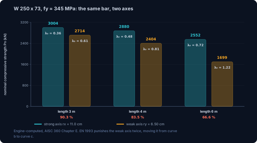
Run the same W 250 x 73 about both axes and the asymmetry from the stiffness section shows up as capacity:
| Length | Strong axis λ₀ | Strong axis Pn | Weak axis λ₀ | Weak axis Pn | Weak / strong |
|---|---|---|---|---|---|
| 3 m | 0.361 | 3004 kN | 0.611 | 2714 kN | 90.3 % |
| 4 m | 0.481 | 2880 kN | 0.814 | 2404 kN | 83.5 % |
| 6 m | 0.721 | 2552 kN | 1.221 | 1699 kN | 66.6 % |
AISC 360 and NBR 8800 handle this with one curve and let the slenderness do the work: the weak axis has a smaller radius of gyration, so it lands further along the same curve. That is the whole story for those two codes.
EN 1993-1-1 goes further, and this is where the physics from earlier becomes a table entry. It selects a different curve per axis, per shape proportion, per flange thickness and per steel grade, and the selection is a direct translation of the residual-stress pattern. For rolled I sections in S235 to S420:
| Shape | Buckling about y-y | Buckling about z-z |
|---|---|---|
| h/b > 1.2, tf ≤ 40 mm | curve a (α = 0.21) | curve b (α = 0.34) |
| h/b ≤ 1.2, tf ≤ 100 mm | curve b (α = 0.34) | curve c (α = 0.49) |
Our shape has h/b = 0.996 and tf = 14.2 mm, so it takes curve b about the strong axis and curve c about the weak axis. At 6 m that means 2448 kN strong and 1344 kN weak: the weak axis is punished twice, once by its larger slenderness and again by being moved to a worse curve. The five curves are the same formula with five values of the imperfection factor α: 0.13, 0.21, 0.34, 0.49 and 0.76 for a0, a, b, c and d. At λ₀ = 1 they give χ = 0.725, 0.666, 0.597, 0.540 and 0.467, a spread of 36 % between the best and the worst shape at identical slenderness.
A note on how the CalcSteel engine handles this today: its EN 1993 check uses curve b (α = 0.34) as a single default for every section, so the curve c numbers quoted above are the same closed-form expression evaluated with α = 0.49, the value Table 6.2 assigns to this shape about z-z. The AISC 360 and NBR 8800 numbers in this article all come straight from the engine.
Try it on your own column
Put your own section and effective length into the calculator below and watch the two answers separate. The Euler critical load is the classical ceiling from this article; the AISC 360 and NBR 8800 capacities are the ceiling minus everything residual stress and out-of-straightness take away.
The gap is worth reading as a diagnostic. If your column comes back near λ₀ = 1, you are standing on the worst point of the curve and roughly a third of the classical capacity is gone. Bracing the weak axis to move the column off that point is often cheaper than upsizing the section, because it moves you down the λ₀ scale into the region where the penalty shrinks fast.
End conditions (buckling case)
Pinned – Pinned
Cross-section
Slenderness KL/r
134.7
limit 200 · OK
Euler Pcr (elastic)
310.7 kN
Fe = 108.9 MPa
AISC 360 φcPn
245.2 kN
Fcr = 95.5 MPa · elastic
NBR 8800 Nc,Rd
247.7 kN
χ = 0.382 · λ₀ = 1.52
Code vs code — same column
Nc,Rd / φcPn = 1.010
Both codes share the 0.658 / 0.877 buckling curve — the ~1% gap is purely φc = 0.90 (AISC) vs 1/γa1 = 0.909 (NBR).
Demand check — Nd = 150 kN
Step-by-step derivation — live for YOUR column
IPE 200 · L = 3 m · K = 1 · fy = 250 MPa
- 1
Slenderness ratio
λ = K·L/r = 1 × 3000 / 22.28 mm
λ = 134.7 (≤ 200 ✓)
- 2
Euler elastic buckling stress and load
Fe = π²E/λ² = π² × 200,000 / 134.7² · Pcr = Fe·A = Fe × 2854 mm²
Fe = 108.9 MPa · Pcr = 310.7 kN
- 3
Buckling regime (AISC E3)
4.71·√(E/fy) = 4.71·√(200,000/250) = 133.2 < λ = 134.7
elastic buckling → use E3-3 (0.877·Fe)
Elastic range: capacity no longer depends on fy — only geometry (r, K, L) helps.
- 4
AISC 360 critical stress and design capacity
Fcr = 0.877 · Fe = 0.877 × 108.9 = 95.5 MPa · φcPn = 0.9 × Fcr × A
Pn = 272.5 kN · φcPn = 245.2 kN
- 5
NBR 8800 reduction factor and design capacity
λ₀ = √(fy/Fe) = 1.515 > 1.5 → χ = 0.877/λ₀² = 0.382 · Nc,Rd = χ·A·fy/1.1
Nc,Rk = 272.5 kN · Nc,Rd = 247.7 kN
Same 0.658/0.877 curve as AISC — the ~1% difference is φc = 0.90 vs 1/γa1 = 0.909.
Sections that work — 3 lightest of 612 catalog profiles carrying Nd = 150 kN at L = 3 m, K = 1
| Section | kg/m | φcPn (kN) | Nc,Rd (kN) | Util. | |
|---|---|---|---|---|---|
| lightestSHS 80x4 | 9.2 | 164 | 166 | 91% | |
| HSS 76x76x4.8 | 9.9 | 165 | 167 | 91% | |
| CHS 88.9x5 | 10.3 | 172 | 174 | 87% |
Pass criterion: φcPn ≥ Nd (AISC 360 LRFD) AND Nc,Rd ≥ Nd (NBR 8800) AND KL/r ≤ 200, using each section's tabulated-mass area and minimum radius of gyration.
Buckling curve — IPE 200, fy = 250 MPa
Capacity of IPE 200 by unbraced length — K = 1, fy = 250 MPa
| L (m) | KL/r | Pcr Euler (kN) | φcPn AISC (kN) | Nc,Rd NBR (kN) | Regime |
|---|---|---|---|---|---|
| 1 | 45 | 2,796 | 577 | 583 | inelastic |
| 2 | 90 | 699 | 419 | 423 | inelastic |
| 3◀ yours | 135 | 311 | 245 | 248 | elastic |
| 4 | 180 | 175 | 138 | 139 | elastic |
| 5 | 224 ⚠ | 112 | 88 | 89 | elastic |
| 6 | 269 ⚠ | 78 | 61 | 62 | elastic |
| 7 | 314 ⚠ | 57 | 45 | 45 | elastic |
| 8 | 359 ⚠ | 44 | 34 | 35 | elastic |
| 9 | 404 ⚠ | 35 | 27 | 28 | elastic |
| 10 | 449 ⚠ | 28 | 22 | 22 | elastic |
Where 0.658 and 0.877 actually came from
Every engineer who has used AISC 360 has typed 0.658 and 0.877 without being told what they are. They are not derived constants. They are calibration coefficients, and the calibration was anchored on residual stress.
The lineage starts with the CRC parabola, the column formula in AISC ASD until 1989. It was built on an explicit assumption: the compressive residual stress at the flange tips is 0.5 fy, so the column stays fully elastic only up to an applied stress of fy/2, and above that the section yields progressively. That assumption produces
Fcr = fy·[1 − fy·λ²/(4π²E)], valid up to Cc = √(2π²E/fy)
and it has a signature: at λ = Cc the parabola equals exactly fy/2. For 345 MPa steel, Cc = 107.0, and the check confirms the parabola lands on 0.5 fy there to nine decimal places. The 0.5 fy residual-stress assumption is not hidden in the formula; it is the formula.
When AISC moved to LRFD in 1986, the parabola was replaced by an exponential fitted to test data and to the SSRC column curves, which had been produced by analysing columns with measured residual stress patterns together with initial out-of-straightness. The derivation is documented in the AISC Engineering Journal: the inelastic coefficient was set at λ = 1.0 to land on a target Fcr/fy of about 0.56 with φ = 0.85, which computes to 0.6589; the elastic coefficient came from matching the two branches at λ = 1.5, which computes to 0.8774; and the crossover was placed at λ = 1.5 specifically "to approximate the historic ASD matching of elastic and inelastic curves at a stress level of Fy/2".
So the modern curve inherited its crossover from the old parabola, and the old parabola got that point from assuming 0.5 fy of residual stress. NBR 8800 adopted the same pair of expressions. When you type 0.658 into a spreadsheet, you are typing a number whose ancestry runs back to how fast a flange tip cools.
It is not only columns
Once you can see residual stress, it turns up in several places that are usually taught as unrelated rules.
- Lateral-torsional buckling. AISC 360 Chapter F builds the inelastic LTB range on 0.7Fy, and the limiting length Lr is the unbraced length at which elastic LTB reaches that stress. The 0.7 is 1 − 0.3: the same 0.3Fy compressive residual stress at the flange tips, now reducing the moment at which the compression flange starts to yield. Same physics, different limit state.
- Cutting and drilling. Residual stress is in equilibrium with itself. Remove material and you remove part of that equilibrium, and the piece moves to find a new one. This is why coping a beam flange, flame-cutting a long strip off a plate or drilling a dense bolt pattern can leave a member visibly out of straight, with nobody having loaded it. Fabricators know this as a sequencing problem long before it is a stress problem.
- Welded shapes. Welding creates a much sharper thermal cycle than rolling, and the residual stress near a weld can approach yield. Welded I sections generally get worse buckling curves than rolled ones of the same proportions. There is a good counter-example: plates with flame-cut edges finish with tension at the edges, because the cut edge is heated and cools last, and a welded section built from flame-cut plate buckles better about the weak axis than one built from mill-edge plate. The manufacturing route, not the geometry, decides.
- Cold-formed sections. The residual stress there is a different animal, dominated by bending through the thickness from the forming rolls rather than by cooling. That is one of the reasons cold-formed steel has its own specification family and its own strength method rather than borrowing the hot-rolled curves.
- Heavy shapes. Thicker material cools more unevenly, so the residual stress gets worse as the section gets heavier. EN 1993 tracks this explicitly: past a flange thickness of 100 mm, a rolled I section drops to curve d about both axes, α = 0.76, the worst curve in the table.
Six ways this goes wrong in practice
- Sizing a column with the Euler load. Euler is an upper bound that no real column reaches. At λ₀ = 1 it overstates the capacity by 34 %, and that is before any resistance factor. Use it to understand the problem, never to size the member.
- Assuming a heavier section is safer against this effect. It is the opposite. Thicker flanges cool more unevenly and carry higher residual stress, which is why the code curves get worse with flange thickness, not better.
- Treating the two axes as one check with a different length. True in AISC and NBR, false in EN 1993, where the weak axis is also moved to a worse curve. Running a Eurocode job with one curve for both axes overstates the weak-axis capacity of a wide shape by around 10 % at λ₀ = 1, and considerably more further along.
- Concluding that self-equilibrating means harmless. It does mean the squash load is unchanged, and that is exactly the trap. The moment stability enters, an internally balanced stress field becomes a stiffness problem.
- Ignoring what fabrication does to a straight member. Flame cutting, heavy welding and unbalanced material removal all disturb a locked-in equilibrium, and the member moves. Straightening it afterwards adds yet more residual stress.
- Reading a low utilisation as a comfortable margin. A column at 50 % of its squash load already has yielded flange tips. Nothing on a stress plot shows it, and the stiffness that the next load increment will need is already reduced.
The honest summary is short. The column curve is not the Euler curve because the steel was not neutral when you got it. It came pre-stressed by its own cooling, it starts yielding at half the load you would expect, it loses its weak-axis stiffness three times faster than its strong-axis stiffness, and the codes have been quietly carrying that correction for you since the 1960s.
Sources
- 1.Hibbeler, Mechanics of Materials (Resistência dos Materiais), chapters on axial load (residual stress after inelastic loading) and buckling of columns
- 2.ECCS (1984), Ultimate Limit State Calculation of Sway Frames with Rigid Joints: the residual stress model for hot-rolled I sections, 0.3 fy for h/b > 1.2 and 0.5 fy for h/b ≤ 1.2
- 3.EN 1993-1-1 Eurocode 3, clause 6.3.1 and Tables 6.1 and 6.2: buckling curves a0 to d, imperfection factors and curve selection by h/b, flange thickness, grade and axis
- 4.AISC 360 Specification, Chapter E (flexural, torsional and flexural-torsional buckling) and Chapter F (the 0.7Fy limit behind Lr)
- 5.Tide, R. H. R. (2001), "A Technical Note: Derivation of the LRFD Column Design Equations", AISC Engineering Journal, Third Quarter 2001
- 6.ABNT NBR 8800, item 5.3 and Anexo E: the χ curve for compression members
- 7.Structural Stability Research Council, Guide to Stability Design Criteria for Metal Structures: measured residual stresses and the multiple column curves
Try CalcSteel for free
Model, analyze and design steel structures in your browser. No install, no signup.
Open the 3D editor